1. Motivation: sports analytics

We have explored in previous posts how projective geometry can be used to relate two different views of the same planar surface. The mapping is encoded in a $3 \times 3$ matrix called the homography matrix, which can be estimated from point correspondences between both views. Once the homography is known, different geometric entities (points, lines, conics) can be projected back and forth between both views.

We have also seen how to relate the 3D world with its 2D projection in the image plane through the camera projection matrix. In particular, we have shown how to calibrate the camera intrinsics and retrieve the camera pose solely using information extracted from the captured image.

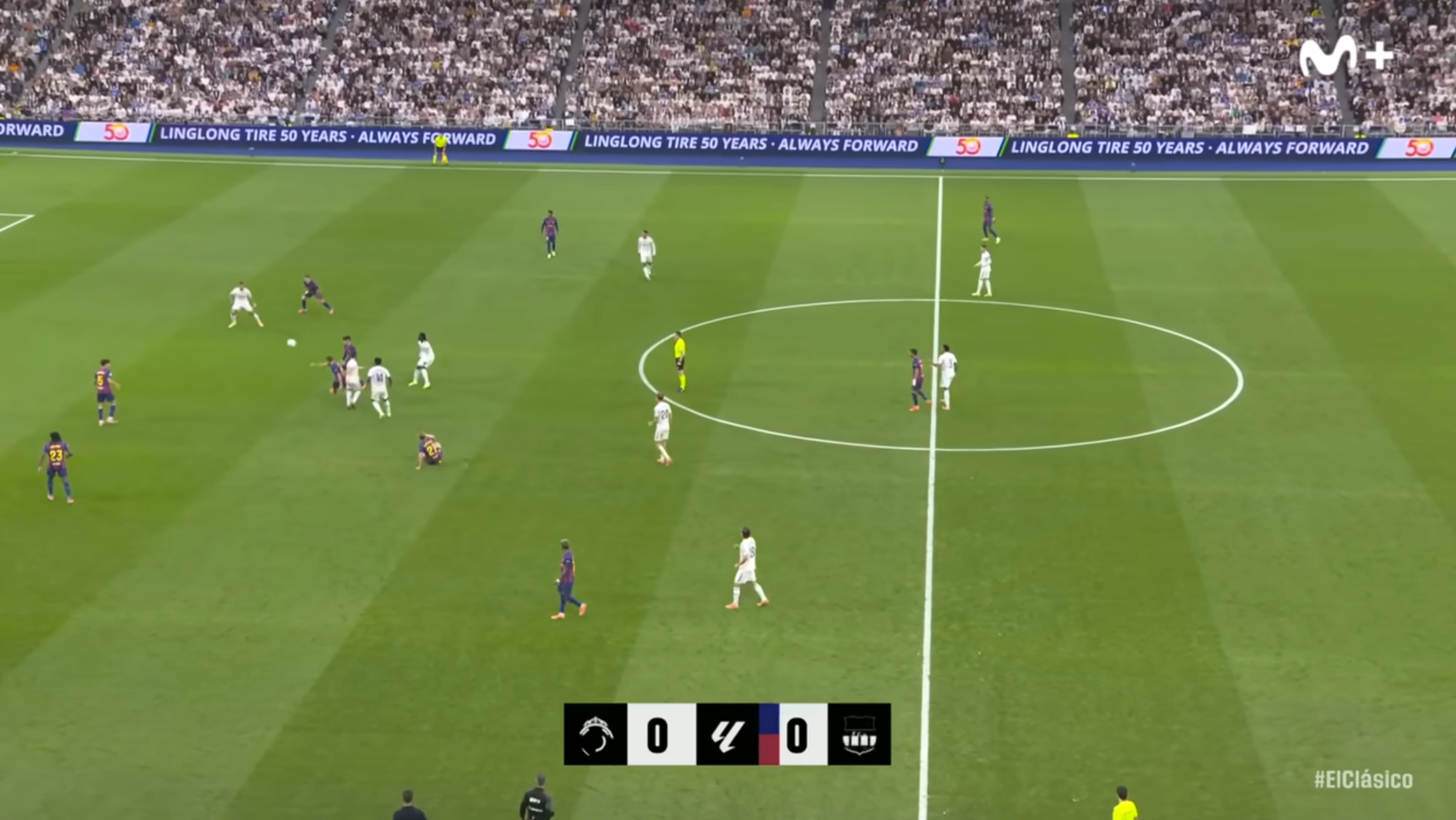
Now it is time to wonder: How about 3D objects? Like a ball in a sports game. It can be modelled as a sphere in 3D space, but how do we project it? And more importantly, how do we retrieve its 3D location from its 2D projection in the image? Take the image below, would you be able to tell if the ball is on the ground or bouncing a few feet above it?

2. Projecting a sphere: from 3D to 2D

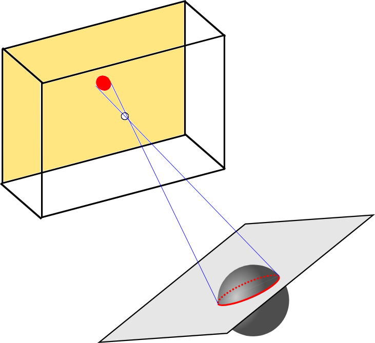
When a 3D object is projected onto the image plane, its 2D contour corresponds to the projection of the outline of the object. More specifically, the outline is defined by the set of points where the projection rays arising from the camera center are tangent to the object surface. Let us take the case of a sphere with radius $R$ to see how its projection is formed:

1. Trace the projection rays from the camera center to the sphere surface such that they are tangent to the sphere.
2. These rays form a right circular cone, with the camera center as its apex.
3. All points of tangency lie in a 2D plane, whose intersection with the sphere gives us the outline.
4. The intersection between the 2 plane and the sphere is the circle of tangency. It has radius $r$, with $r<R$.
5. Finally, the projection of this circle onto the image plane gives us a conic section.

So how do we model this mathematically? A 3D sphere can be represented in homogenous coordinates by a $4 \times 4$ matrix $Q$. All points $P=[X, Y, Z, 1]^T$ that lie on the sphere satisfy the equation:

$$ \begin{equation} P^T\cdot Q\cdot P = 0 \end{equation} $$

If you recall from our previous post, there is an equivalent parametrization given by the dual quadric $\Theta$, which for a sphere is simply $\Theta = Q^{-1}$. All planes $\Pi$ that are tangent to the sphere satisfy:

$$ \begin{equation} \Pi^T\cdot \Theta \cdot \Pi = 0 \end{equation} $$

The projection of the sphere onto the image plane is a conic section represented by a $3 \times3$ matrix $C$. Similarly to the 3D case, its dual conic $D = C^{-1}$ represents all lines $l$ that are tangent to the conic:

$$ \begin{equation} l^T\cdot D \cdot l = 0 \end{equation} $$

We know a line $l$ back projects to a plane $\Pi=H^T\cdot l$, where $H$ is the camera projection matrix. If we were to back project all lines tangent to the conic, we would obtain all planes tangent to the sphere. Therefore, they must satisfy:

$$ \begin{equation} \begin{split} \Pi^T\cdot \Theta \cdot \Pi &= (H^T\cdot l)^T \cdot \Theta \cdot (H^T\cdot l) \\ &= l^T \cdot (H \cdot \Theta \cdot H^T) \cdot l \end{split} \end{equation} $$

So in order to satisfy the equation of tangency for the conic, we can simply take:

$$ \begin{equation} \boxed{ D = H \cdot \Theta \cdot H^T } \end{equation} $$

3. Back-projecting a conic: from 2D to 3D

So can we go back? Given the conic $C$ in the image, can we retrieve the dual quadric $\Theta$ of the sphere in 3D space? This is what we are set to do in this section. To get some intuition of why this may be feasible, take a look at the interactive figure below.

We have a basket ball and the slider allows us to change its distance from the camera along its optical axis. As we move the ball closer or further away, notice how its projection onto the image plane (orange) changes in size. If we were just dealing with a point, we would not be able to tell its distance from the camera just by looking at its projection. However, since we have a sphere with known radius, we can exploit the size of its projection to infer its 3D location!

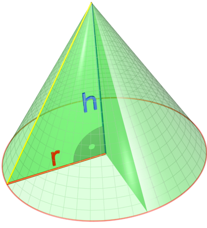
3.1. Parametrizing a cone

Let us start by noticing a conic maps back to a cone. How do we parametrize a cone? Let us assume the cone has its apex at the origin and its axis aligned with the $Z$ axis. Then, we can define a cone by the following equations:

$$ \begin{equation} \begin{split} \frac{X^2}{a^2} + \frac{Y^2}{b^2} &= R^2 \\ R &= \frac{Z}{c} \end{split} \end{equation} $$

which can be rearranged to give:

$$ \begin{equation} \frac{X^2}{a^2} + \frac{Y^2}{b^2} - \frac{Z^2}{c^2} = 0 \end{equation} $$

or in matrix form:

$$ \begin{equation} \begin{bmatrix}X & Y & Z \end{bmatrix}\cdot \begin{bmatrix} \frac{1}{a^2} & 0 & 0 \\ 0 & \frac{1}{b^2} & 0 \\ 0 & 0 & -\frac{1}{c^2} \\ 0 & 0 & 0 \end{bmatrix}\cdot \begin{bmatrix}X \\ Y \\ Z \end{bmatrix} = 0 \end{equation} $$

or more succinctly:

$$ \begin{equation} P^T \cdot Q_{\text{co}} \cdot P = 0 \end{equation} $$

So basically we have a cross section of an ellipse that scales linearly with $Z$. The parameters $a$, $b$ and $c$ define the shape of the cone. We can distinguish between:

1. Elliptical cones: when $a \neq b$
2. Circular cones: when $a = b$

Any rotation, $R$, can be applied to the cone, transforming its matrix into:

$$ \begin{equation} Q_{\text{co}}’ = R^T \cdot Q_{\text{co}} \cdot R \end{equation} $$

We can also translate the cone, which would require switching to homogeneous coordinates. But if we assume the apex is at the origin, we can skip this step for now.

3.2. Back-projecting the conic

We know a 3D point $P$ gets projected to $p = H \cdot P$. Furthermore, a point $p$ lies on the conic if it satisfies:

$$ \begin{equation} p^T \cdot C \cdot p = 0 \end{equation} $$

so points $P$ that project to the conic must satisfy:

$$ \begin{equation} P^T \cdot H^T \cdot C \cdot H \cdot P = 0 \end{equation} $$

If we take $Q_{\text{co}} = H^T \cdot C \cdot H$, we see that points $P$ that lie on the cone satisfy:

$$ \begin{equation} P^T \cdot Q_{\text{co}} \cdot P = 0 \end{equation} $$

And we can verify that the vertex $V$ of the cone corresponds to the camera center by checking the vertex condition $Q_{\text{co}} \cdot V = 0`. Recall the homography matrix is defined as:

$$ \begin{equation} H=K\cdot R^T \cdot \left[\; I\;\; | \;\;-\vec{t}\;\;\right ] \end{equation} $$

where $\vec{t}$ is the camera center. So if we take $V = [\vec{t}, 1]^T$, we have:

$$ \begin{equation} Q_{\text{co}} \cdot V = H^T \cdot C \cdot H \cdot V = 0 \end{equation} $$

Importantly, the cone matrix $Q_{\text{co}}=H^T \cdot C \cdot H$ is a $4 \times 4$ matrix, while our previous parametrization of the cone was a $3\times 3$ matrix. This is a more general representation that allows for translation of the cone apex. However, there is a trick we can use to simplify this expression. We can shift the coordinate system to the camera center. This way, our homography matrix becomes:

$$ \begin{equation} H’ = K \cdot R^T \cdot \left[\; I\;\; | \;\; 0\;\;\right ] \end{equation} $$

and the cone matrix simplifies to:

$$ \begin{equation} Q_{\text{co}}’ = \begin{bmatrix} RK^T \\ 0 \end{bmatrix} \cdot C \cdot \begin{bmatrix} KR^T & 0 \end{bmatrix}= \begin{bmatrix} RK^T C KR^T & 0 \\ 0 & 0 \end{bmatrix} \end{equation} $$

so it is fully defined by the $3\times 3$ matrix as expected.

3.3. Dealing with noise

We have started from a 3D sphere (the ball) and projected it onto the image plane, obtaining a 2D conic. Then, in our aim to retrieve the 3D location of the ball, we have back-projected the conic to obtain a 3D cone. By construction, this cone must be a circular cone since it was generated by the projection rays tangent to a sphere.

Nonetheless, in practice the conic we obtain from the image could be contaminated by noise due to different factors (imperfect camera calibration, imperfect homography estimation, imperfect conic fitting to the projected ball contour, etc). Therefore, when we back-project the conic to 3D space, the resulting cone may not be a right circular cone.

To solve this, we can try to find the closest circular cone to the back-projected cone. This is closely related to the Procrustes problem in linear algebra, where we try to find the closest orthogonal matrix to a given matrix.

Let us assume the back-projected cone is defined by the $3\times 3$ matrix $\hat{Q}$. We saw earlier how a cone with apex at the origin can be parametrized by a matrix $Q$:

$$ \begin{equation} Q = R^T \cdot \Sigma \cdot R \end{equation} $$

where $R$ is a rotation matrix and $\Sigma$ is a diagonal matrix of the form:

$$ \begin{equation} \Sigma = \begin{bmatrix} \lambda_\perp & 0 & 0 \\ 0 & \lambda_\perp & 0 \\ 0 & 0 & \lambda_\parallel \end{bmatrix} \end{equation} $$

with $\lambda_\perp$ and $\lambda_\parallel$ having opposite signs.

So we are looking for the matrices R and $\Sigma$ that minimize

$$ \begin{equation} \min_{R, \Sigma} ||\hat{Q} - R^T \cdot \Sigma \cdot R||_F^2 \end{equation} $$

This expands to:

$$ \begin{equation} \min_{R, \Sigma} ||\hat{Q}||_F^2 - 2\cdot \text{tr}(\hat{Q} \cdot R^T \cdot \Sigma \cdot R) + ||\Sigma||_F^2 \end{equation} $$

If we focus on $R$, this is equivalent to maximizing

$$ \begin{equation} \max_{R} \text{tr}(\hat{Q} \cdot R^T \cdot \Sigma \cdot R) \end{equation} $$

We can compute the SVD of $\hat{Q}$ as $\hat{Q} = U \cdot D \cdot U^T$, where $D$ is a diagonal matrix with the eigenvalues of $\hat{Q}$. Then, we can rewrite the maximization as:

$$ \begin{equation} \max_{R} \text{tr}(U \cdot D \cdot U^T \cdot R^T \cdot \Sigma \cdot R) \end{equation} $$

Given the cyclic property of the trace, we can rearrange the terms to get:

$$ \begin{equation} \max_{R} \text{tr}(D \cdot U^T \cdot R^T \cdot \Sigma \cdot R \cdot U) \end{equation} $$

and if we define $M = R \cdot U$, we have:

$$ \begin{equation} \max_{M} \text{tr}(D \cdot M^T \cdot \Sigma \cdot M) \end{equation} $$

From Von Neumann’s trace inequality, we know that

$$ \begin{equation} \text{tr}(A \cdot B) \leq \sum_i \sigma_i(A) \cdot \sigma_i(B) \end{equation} $$

and the upper bound is attained when $A$ and $B$ are simultaneously diagonalizable, meaning they share the same eigenvectors. In our case, with $\text{tr}(D \cdot (M^T \cdot \Sigma \cdot M))$, $D$ is already diagonal. Therefore, in order for $M^T \cdot \Sigma \cdot M$ to share the same eigenvectors, it must also be diagonal. This is achieved when $M = I$, so

$$ \begin{equation} \boxed{ R = U^T } \end{equation} $$

Now we only need to find the optimal $\Sigma$. Replacing $R$ by $U^T$ in the original minimization, we just need to minimize:

$$ \begin{equation} \min_{\Sigma} ||D - \Sigma||_F^2 \end{equation} $$

or equivalently:

$$ \begin{equation} \min_{\lambda_\perp, \lambda_\parallel} (\lambda_1 - \lambda_\perp)^2 + (\lambda_2 - \lambda_\perp)^2 + (\lambda_3 - \lambda_\parallel)^2 \end{equation} $$

We can solve this by taking derivatives and setting them to zero, obtaining:

$$ \begin{equation} \boxed{ \begin{split} \lambda_\perp &= \frac{\lambda_1 + \lambda_2}{2} \\ \lambda_\parallel &= \lambda_3 \end{split} } \end{equation} $$

4. Retrieving the 3D ball location

We have now all the ingredients to retrieve the 3D location of the ball. We have back-projected the conic to obtain a cone in 3D space. We have enforced circularity to obtain a right circular cone. Now, we just need to fit a sphere of known radius $R$ inside that cone such that it is tangent to it.

There are infinitely many spheres inside that cone tangent to it. But here is the catch: if we know the radius of the sphere $R$, there is only one sphere of radius $R$ that is tangent to the cone.

Notice how tangency requires:

1. The center of the sphere lies along the axis of the cone.
2. The distance from the center of the sphere to the cone surface is equal to the sphere radius $R$.
3. The cone angle $\theta$ is related to the sphere radius $R$ and the distance from the camera center to the sphere center $d$ by the equation: $\sin(\theta) = \frac{R}{d}$.

The cone angle is directly related to the eigenvalues $\lambda_\parallel$ and $\lambda_\perp$:

$$ \begin{equation} \sin(\theta) = \sqrt{\frac{\lambda_\parallel}{\lambda_\parallel - \lambda_\perp}} \end{equation} $$

So we can retrieve the distance from the camera center to the sphere center as:

$$ \begin{equation} d = \frac{R}{\sin(\theta)} = R\cdot{\sqrt{\frac{\lambda_\parallel - \lambda_\perp}{\lambda_\parallel}}} \end{equation} $$

Last, recall that we have shifted the coordinate system to the camera center. Therefore, to retrieve the sphere center $P_0$in world coordinates, we need to:

$$ \begin{equation} P_0 = \vec{t} + d \cdot \vec{v} \end{equation} $$

where $\vec{t}$ is the camera center in world coordinates and $\vec{v}$ is the unit vector along the cone axis direction (i.e., $\vec{u_3}$ from the SVD of the cone matrix).

The interactive demo below allows you to move around the ball in 3D space and see how its projection changes in the image. It estimates its 3D location in the background following the steps we have just described, and displays the estimated location.

5. Conclusion

In this post we have shown how the 3D location of a sphere with known radius can be retrieved from a single frame displaying its projection onto the image plane. In summary:

1. A 3D sphere projects to a conic in the image plane that corresponds to the projection of the circle of tangency between the sphere and the cone formed by the projection rays tangent to the sphere. We know how to obtain that 2D conic: $$ \begin{equation} D = H \cdot \Theta \cdot H^T \end{equation} $$
2. Once that 2D conic is fitted in the image, it can be back-projected to a cone in 3D space with apex at the camera center. We know how to obtain that 3D cone: $$ \begin{equation} Q_{\text{co}} = H^T \cdot C \cdot H \end{equation} $$
3. The vertex of the cone corresponds to the camera center $\vec{t}$, so if we shift the coordinate system to the camera center: $$ \begin{equation} Q_{\text{co}}’ = \begin{bmatrix} Q’ & 0 \\ 0 & 0 \end{bmatrix} \end{equation} $$
4. The SVD of the $3\times 3$ matrix $Q’$ can be computed as $Q’ = U \cdot D \cdot U^T$. $D$ satisfy $D = \text{diag}(\lambda_1, \lambda_2, \lambda_3)$ with $\lambda_1$, $\lambda_2$ sharing the same sign and $\lambda_3$ having the opposite sign. $U$ is a rotation matrix $U=[\vec{u_1}, \vec{u_2}, \vec{u_3}]$, where $\vec{u_3}$ is the cone axis direction.
5. Circularity can be enforced by adjusting so $Q’’ = R^T \cdot \Sigma \cdot R$, where $R = U^T$ and $\Sigma=\text{diag}(\lambda_\perp, \lambda_\perp, \lambda_\parallel)$ with $\lambda_\perp = (\lambda_1 + \lambda_2)/2$ and $\lambda_\parallel = \lambda_3$.
6. Finally, the distance from the camera center to the sphere center can be retrieved as: $$ \begin{equation} d = R\cdot{\sqrt{\frac{\lambda_\parallel - \lambda_\perp}{\lambda_\parallel}}} \end{equation} $$ and the sphere center in world coordinates is: $$ \begin{equation} P_0 = \vec{t} + d \cdot \vec{u_3} \end{equation} $$

Note: you can give it a try by simply running this script. In order to do so, just install the repository (poetry install) and then run

poetry run python -m projective_geometry locate-ball-3d 3 5 6

where 3 5 6 are the $X, Y, Z$ coordinates of the ball in meters. The script will simulate the projection of the ball onto the image plane and then retrieve its 3D location from that projection.

6. References

1. Richard Hartley and Andrew Zisserman (2000), Page 143, Multiple View Geometry in Computer Vision, Cambridge University Press.
2. Wikipedia. Cone
3. Wikipedia. Von Neumann’s trace inequality
4. Wikipedia. Procrustes problem