Table of Contents

1. Pinhole camera model

When we capture something on camera, there is an interesting phenomenon going on: compression. We are taking a photograph of a 3D world, and capturing it in a 2D image. This 3D→2D space mapping inevitably leads to information loss. There are multiple locations in the 3D world that project exactly to the same position in the 2D image. Nonetheless, this observation should not come as a surprise to anyone: it is precisely the reason occlusions take place. Multiple objects at different places end up in the same location when viewed through a 2D projection, be it a film or our retina.

So how do we model that 3D→2D mapping? That is what projective geometry is all about. To understand this transform, let us start with the ideal pinhole camera model, illustrated below:

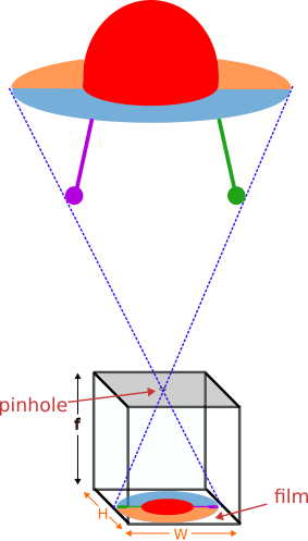
In this setup, the camera consists of a simple dark box with a small aperture (termed pinhole), located in its front, and a film on its rear wall, with dimensions (W, H). The distance between the pinhole and the film is known as the focal length (f).

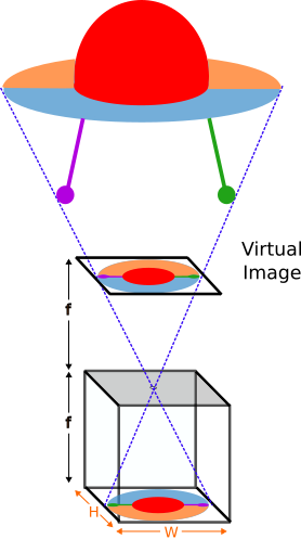
The image is formed when the light rays enter it through the pinhole (which we will assume of infinitesimal radius) and are captured by the photographic material the film is composed of. This way, an inverted image is obtained, which can be flipped in a post-processing step. Moreover, this is equivalent to forming a virtual image in front of the camera, at a distance f from the pinhole.

2. Intrinsic matrix

2.1. Setup

In order to characterize the projection, let us start by defining the two system of coordinates involved in the transform:

• 3D World: we define the origin of coordinates located at the camera pinhole. Furthermore, the cartesian axes will also be aligned with the camera axes.
• 2D Image: we define the origin of coordinates located at the bottom-left corner of the virtual image.

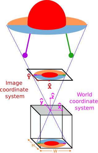
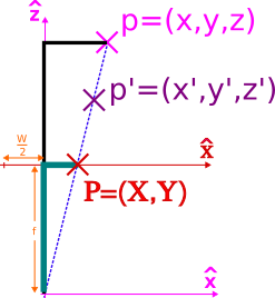
Given these arbitrary definitions, we can now determine where a point $p=(x, y, z)$ will be projected in the image. To do so, we just need to recall that the projection $P=(X, Y)$ is found at the intersection between the plane containing the virtual image, and the ray passing through both the point p and the pinhole $o=(0, 0, 0)$.

For simplicity, let us focus on how the projection takes place for the horizontal dimension $x$:

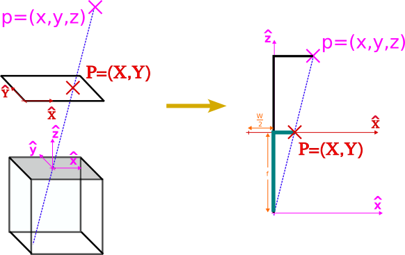
We can observe that there are two similar triangles (black and green) on the right image. Therefore, the rate between the lengths of their sides is preserved:

$$ \begin{equation}\frac{z}{x} = \frac{f}{X-\frac{W}{2}}\end{equation} $$

or equivalently

$$ \begin{equation}f\cdot x+\frac{W}{2}\cdot z=X \cdot z\end{equation} $$

We can derive the projection along the y dimension in an analogous fashion, resulting in:

$$ \begin{equation}f\cdot y+\frac{H}{2}\cdot z=Y \cdot z\end{equation} $$

2.2. Homogeneous coordinates

At this point, it is worth wondering: can we express the previous equations as a matrix product?

$$ \begin{equation} \begin{bmatrix} f & 0 & \frac{W}{2}\\ 0 & f & \frac{H}{2}\\ 0 & 0 & 1 \end{bmatrix} \cdot \begin{bmatrix} x \\ y \\ z \end{bmatrix} = \begin{bmatrix} X\cdot z \\ Y\cdot z \\ z \end{bmatrix} \end{equation} $$

It is almost what we want, but we have an extra scaling factor on the right hand-side

$$ \begin{equation} \begin{bmatrix} f & 0 & \frac{W}{2}\\ 0 & f & \frac{H}{2}\\ 0 & 0 & 1 \end{bmatrix} \cdot \begin{bmatrix} x \\ y \\ z \end{bmatrix} = z\cdot \begin{bmatrix} X \\ Y \\ 1 \end{bmatrix} \end{equation} $$

And here is where homogeneous coordinates show up. For a point $\vec{P}=[X,Y]^T$, its homogeneous coordinates can be defined as

$$ \begin{equation} \vec{P_H}=\begin{bmatrix} s\cdot X \\ s\cdot Y \\ s \end{bmatrix} = s\cdot \begin{bmatrix} X \\ Y \\ 1 \end{bmatrix} \end{equation} $$

Leveraging this definition, we can express the projection as

$$ \begin{equation}K\cdot \vec{p}=\vec{P}_H \end{equation} $$

where $K$ is defined as the intrinsic matrix

$$ \begin{equation} K=\begin{bmatrix} f & 0 & \frac{W}{2}\\ 0 & f & \frac{H}{2}\\ 0 & 0 & 1 \end{bmatrix} \end{equation} $$

and $\vec{p}$ corresponds to the 3D world point

$$ \begin{equation} \vec{p}=\begin{bmatrix} x\\ y\\ z \end{bmatrix} \end{equation} $$

ImportantIy, homogenous coordinates are defined up to a scale. Why is that the case? Going back to the introduction, we stated that there was a compression involved in projective geometry. We are capturing a 3D world into a 2D image. That implies that there is an infinite set of aligned points (i.e. a line) in the 3D world that are mapped exactly to the same location in image space. Take a look at the image below

Once again, due to the similarity of the triangles involved, we know that

$$ \begin{equation}\frac{z}{z’} = \frac{x}{x’} = \frac{y}{y’} = s \end{equation} $$

If we plug in our matrix equation both $\vec{p}$ and $\vec{p’}$, we will obtain

$$ \begin{equation} \vec{P_H}=\begin{bmatrix} f\cdot x + \frac{W}{2}\cdot z \\ f\cdot y + \frac{H}{2}\cdot z \\ z \end{bmatrix} \end{equation} $$

and

$$ \begin{equation} \vec{P_H}’=\begin{bmatrix} f\cdot x’ + \frac{W}{2}\cdot z’ \\ f\cdot y’ + \frac{H}{2}\cdot z’ \\ z’ \end{bmatrix} \end{equation} $$

It is clear these two vectors are not the same. However, they are proportional

$$ \begin{equation} \vec{P_H}’=s\cdot\vec{P_H} \end{equation} $$

Consequently, in homogeneous coordinates, they represent exactly the same point in image space! And how do we obtain its image coordinates $\vec{P}=[X,Y]^T$? Following the definition in eq.(6), we simply need to divide by the scale factor encoded in the last dimension:

$$ \begin{equation} X=\frac{{P_H}_x}{{P_H}_z} \end{equation} $$

$$ \begin{equation} Y=\frac{{P_H}_y}{{P_H}_z} \end{equation} $$

2.3. Accounting for distortions

2.3.1. Digital images

So far, we have assumed we had an analog camera, so the image coordinates lived in a continuous space. However, most often we deal with digital images. Since the information needs to be stored in bits, we need to both discretize the locations at which we sample the image, and quantitize the values we measure.

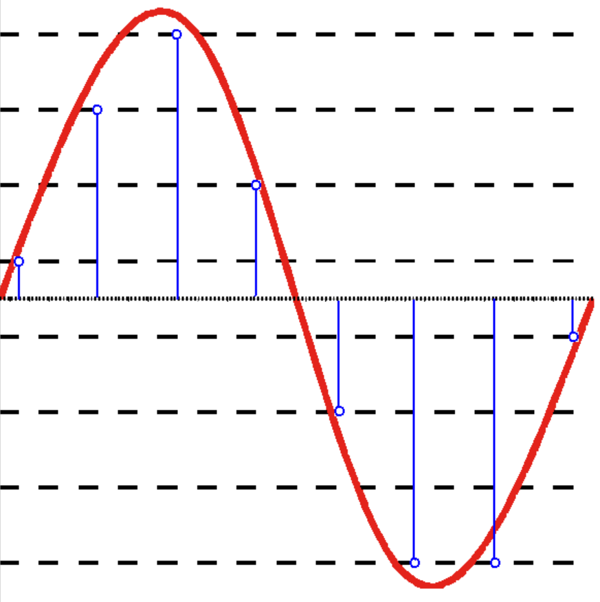
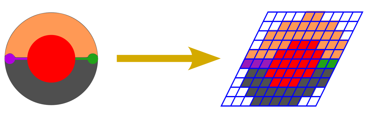
Since we are focused on the spatial mapping, the effect we care about is the discretization that takes place in the projected image. If we use squared pixels, we will get something as displayed below:

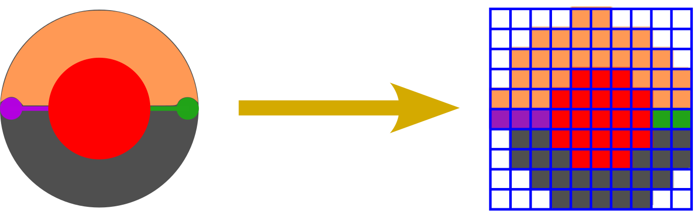
The length of the pixel side is given by the width (height) of the image divided by the number of pixels along the corresponding dimension $N_x$ ($N_y$):

$$ \begin{equation} \Delta=\frac{W}{N_x}=\frac{H}{N_y} \end{equation} $$

We can now express the image coordinates using the pixel length as its units. That is to say, both the image dimensions and the focal length can be defined in pixels:

$$ \begin{equation} f=f_I\cdot\Delta,\;\;\;\;\;\;\;\; W=W_I\cdot\Delta,\;\;\;\;\;\;\;\; H=H_I\cdot\Delta \end{equation} $$

As a result, if we want to obtain the projected coordinates in this discretized image space, we simply need to tweak slightly our intrinsic matrix:

$$ \begin{equation} K=\begin{bmatrix} \frac{f}{\Delta} & 0 & \frac{W}{2\Delta}\\ 0 & \frac{f}{\Delta} & \frac{H}{2\Delta}\\ 0 & 0 & 1 \end{bmatrix} = \begin{bmatrix} f_I & 0 & \frac{W_I}{2}\\ 0 & f_I & \frac{H_I}{2}\\ 0 & 0 & 1 \end{bmatrix} \end{equation} $$

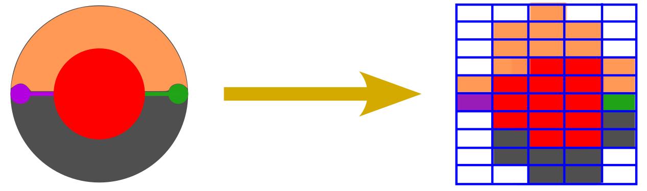
So what happens if instead we have non-squared pixels?

$$ \begin{equation} \Delta_x = r\cdot\Delta_y \end{equation} $$

Well, that is how we end up with two different focal lengths along each dimension:

$$ \begin{equation} W=W_I\cdot\Delta_x \end{equation} $$

$$ \begin{equation} H=H_I\cdot\Delta_y \end{equation} $$

$$ \begin{equation} f=f{_I}_x\cdot\Delta_x \end{equation} $$

$$ \begin{equation} f=f{_I}_y\cdot\Delta_y \end{equation} $$

which leads to the common definition of the intrinsic matrix (we have dropped the subindex $I$ for ease of notation)

$$ \begin{equation} K=\begin{bmatrix} f_x & 0 & \frac{W}{2}\\ 0 & f_y & \frac{H}{2}\\ 0 & 0 & 1 \end{bmatrix} \end{equation} $$

2.3.2. Rephotographing Images

It is common to see an additional parameter in the intrinsic matrix: the skew factor. It accounts for a shearing effect, i.e., image axes not being perpendicular, which results in non-rectangular parallelogrammatic pixels.

Mathematically, it can be modelled by a simple change of basis. Therefore, we just need to find the coefficients of the point expressed in the new basis. Using trigonometry, we can derive.

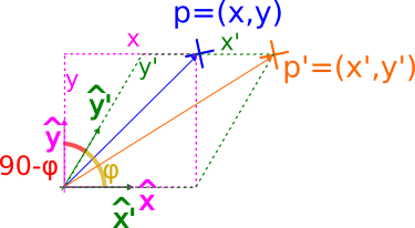
Using trigonometry, we can derive

$$ \begin{equation} \cos(90-\varphi)=\sin(\varphi)=\frac{y}{y’} \; \; \;\rightarrow \; y’=\frac{y}{\sin(\varphi)} \end{equation} $$

$$ \begin{equation} \sin(90-\varphi)=\cos(\varphi)=\frac{x’-x}{y’} \; \; \;\rightarrow \; x’ = x - y’\cdot \cos(\varphi) \end{equation} $$

and combining both equations

$$ \begin{equation} x’ = x - y\cdot\cos(\varphi) / \sin(\varphi) = x - y\cdot\cot(\varphi) \end{equation} $$

or in matrix form

$$ \begin{equation}\begin{bmatrix} x’ \\ y’ \end{bmatrix} =\begin{bmatrix} 1 & -\cot(\varphi) \\ 0 & \frac{1}{\sin(\varphi)} \end{bmatrix} \cdot \begin{bmatrix} x \\ y \end{bmatrix} \end{equation} $$

Overall, there is a nice way to decouple the different transforms we have discussed so far:

1. Scaling: projecting 3D world into 2D image

   $$ \begin{equation} \begin{bmatrix} f_x & 0 & 1\\ 0 & f_y & 1\\ 0 & 0 & 1 \end{bmatrix} \end{equation} $$

2. Shearing: accounting for non-perpendicular axes

   $$ \begin{equation} \begin{bmatrix} 1 & -\cot(\varphi) & 0\\ 0 & \frac{1}{\sin(\varphi)} & 0\\ 0 & 0 & 1 \end{bmatrix} \end{equation} $$

3. Shift: to move the origin of the image space to the bottom-left of the image.

   $$ \begin{equation}\begin{bmatrix} 1 & 0 & \frac{W}{2}\\ 0 & 1 & \frac{H}{2}\\ 0 & 0 & 1 \end{bmatrix} \end{equation} $$

which overall results in the following intrinsic matrix

$$ \begin{equation}K’ =\begin{bmatrix} 1 & 0 & \frac{W}{2}\\ 0 & 1 & \frac{H}{2}\\ 0 & 0 & 1 \end{bmatrix} \cdot \begin{bmatrix} 1 & -\cot(\varphi) & 0\\ 0 & \frac{1}{\sin(\varphi)} & 0\\ 0 & 0 & 1 \end{bmatrix} \cdot \begin{bmatrix} f_x & 0 & 1\\ 0 & f_y & 1\\ 0 & 0 & 1 \end{bmatrix} \end{equation} $$

It can be reduced to

$$ \begin{equation} K’=\begin{bmatrix} f_x & -f_x\cdot\cot(\varphi) & \frac{W}{2}\\ 0 & \frac{f_y}{\sin(\varphi)} & \frac{H}{2}\\ 0 & 0 & 1 \end{bmatrix} \end{equation} $$

or how it is more often presented:

$$ \begin{equation} K’=\begin{bmatrix} f_x & s & \frac{W}{2}\\ 0 & f_y & \frac{H}{2}\\ 0 & 0 & 1 \end{bmatrix} \end{equation} $$

Notice how it is fully characterised with 5 parameters: the focal length along both dimensions $(f_x, f_y)$, the skew factor $s$ and the image size $(W, H)$.

It is worth pointing out that in most cases, the shearing effect is not present. It is very unlikely that a camera is flawed to the point of not having its axes perpendicular. However, it can arise when a picture is retaken and the film of the second camera is not parallel with the image.

3. Extrinsic matrix

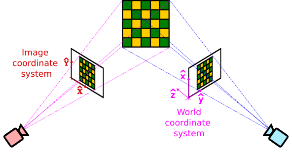
So far, we have assumed our arbitrarily world coordinate system (pink) is perfectly aligned with our camera coordinate system (green), with its origin at the camera pinhole and its Cartesian axes parallel to the camera axes.

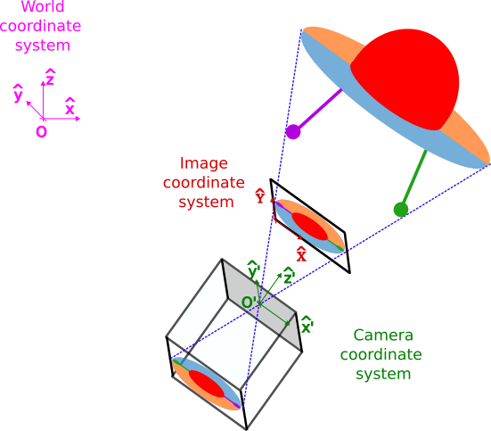
However, when we take photos of videos in the world, we often rotate and/or shift the camera. This results in a camera system that can be derived from the world system by applying two steps sequentially:

1. Rotate the axes by:

   $$ R(\varphi_x,\varphi_y,\varphi_z)\equiv R $$

2. Shift the origin by

   $$ t\vec{}=\begin{bmatrix} t_x \\ t_y \\ t_z \end{bmatrix} $$

These two parameters $(R, \vec{t})$ define the camera pose.

In such a scenario, it might be convenient to have a static coordinate system as a reference, which the camera does not provide anymore. Consequently, it is worth considering: how can we define mathematically the camera projection under these circumstances?

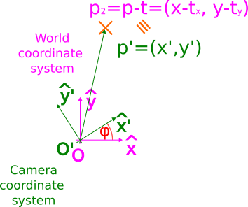
In order to account for this misalignment, it is useful to understand how we can map the coordinates between both coordinate systems. To better understand how that is done, let us simplify to 2D, as depicted in the following figure:

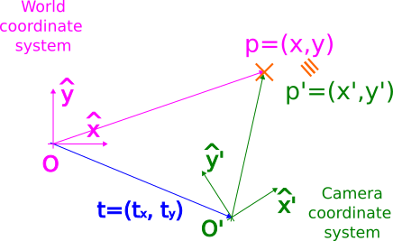
The origin of coordinates in the camera system is located at $\vec{t}=[t_x,t_y]$ w.r.t. the world system. Following this observation, we can infer that in order to align both origin of coordinates $O$ and $O’$, we just need to apply a shift given by the vector $\vec{t}$:

However, we still need to account for the rotation between the axes, given by angle $\varphi$.

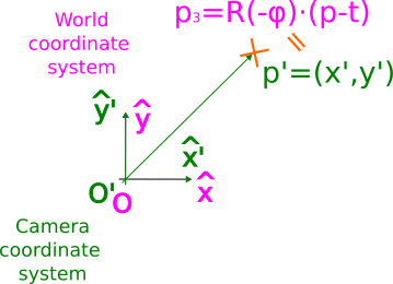
As we can observe, now both systems are perfectly aligned (notice how we used the equal symbol between $p_3$ and $p’$, not just the equivalent symbol). Accordingly, to express a point in the camera system, we just need to apply two steps:

1. Reverse shift:

   $$ \begin{equation} \vec{p}_2=\vec{p}-\vec{t} \end{equation} $$

2. Reverse rotation:

   $$ \begin{equation} \vec{p’}=\vec{p}_3= R^{-1}\cdot\vec{p}_2= R^T\cdot(\vec{p}-\vec{t}) \end{equation} $$

   where we have exploited the fact that rotation matrices are unitary, so their inverse is equal to their transpose.

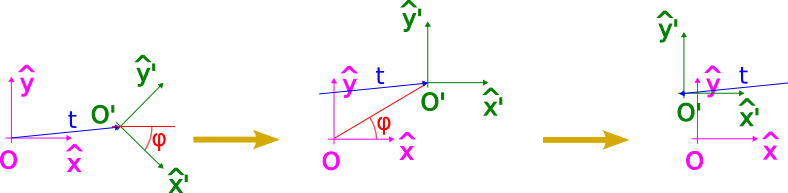
It is worth remarking that order matters!. If we were to rotate first, we would not be rotating around $O’$ as we would hope to in order to align the camera axes, but around $O$, as illustrated below

At this point, it is worth wondering: is there any way we can synthetize the previous equation into a simple matrix product?

$$ \begin{equation} \vec{p’}= \begin{bmatrix} x’ \\ y’ \\ z’ \end{bmatrix} = R^T\cdot \left( \begin{bmatrix} x \\ y \\ z \end{bmatrix} - \begin{bmatrix} t_x \\ t_y \\ t_z \end{bmatrix} \right) \end{equation} $$

It should not come as a surprise to see homogeneous coordinates come to the rescue once again:

$$ \begin{equation} \vec{p_H’}=\begin{bmatrix} x’ \\ y’ \\ z’ \\ 1 \end{bmatrix} = \left[\; R^T\;\; | \;\;-R^T\cdot\vec{t}\;\;\right ]\cdot \begin{bmatrix} x \\ y \\ z \\ 1 \end{bmatrix} =\left[\; R^T\;\; | \;\;-R^T\cdot\vec{t}\;\;\right ]\cdot {p_H} \end{equation} $$

which allows us to define the extrinsic matrix as

$$ \begin{equation} E= \left[\; R^T\;\; | \;\;-R^T\cdot\vec{t}\;\;\right ] \end{equation} $$

In some texts, you might find an equivalent definition given by

$$ \begin{equation} E= \left[\; R’\;\; | \;\;\vec{T}\;\;\right ] \end{equation} $$

where $R’=R^T$ and $\vec{T}=-R^T\cdot\vec{t}$.

To sum up, the extrinsic matrix is fully described by 6 parameters: the 3D location of the camera $(t_x, t_y, t_z)$ and its 3 rotation angles $(\varphi_x,\varphi_y,\varphi_z)$ defining its orientation.

4. Homography matrix

In the light of these definitions, we have all the ingredients to build the $3\times 4$ homography matrix $H$ we were looking for

$$ \begin{equation} H=K\cdot E = \begin{bmatrix} h_{11} & h_{12} & h_{13} & h_{14}\\ h_{21} & h_{22} & h_{23} & h_{24}\\ h_{31} & h_{32} & h_{33} & h_{34}\\ \end{bmatrix} \end{equation} $$

which will allow us to project points from the 3D world into a 2D image

$$ \begin{equation} \vec{P_H}=H\cdot\vec{p_H} \end{equation} $$

or if we expand it

$$ \begin{equation} s\cdot \begin{bmatrix} X \\ Y \\ 1 \\ \end{bmatrix}=\begin{bmatrix} f_x & 0 & \frac{W}{2}\\ 0 & f_y & \frac{H}{2}\\ 0 & 0 & 1 \end{bmatrix} \cdot \begin{bmatrix} r_{11} & r_{12} & r_{13} & T_x\\ r_{21} & r_{22} & r_{23} & T_y\\ r_{31} & r_{32} & r_{33} & T_z\\ \end{bmatrix} \cdot \begin{bmatrix} x \\ y \\ z \\ 1 \ \end{bmatrix} \end{equation} $$

From this definition, we can notice that the process is irreversible, since we can not invert a $3\times 4$ matrix. However, the homography transform can also be used to characterize the mapping between two different 2D planes. This arises when we take two photographs of the same scene from different camera angles for instance, as illustrated below:

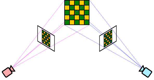
So what can we do in this scenario? Remember we have chosen arbitrarily how to define our coordinate systems. Thus, we can rearrange the 3D world coordinate system to conveniently align with one of the images, such that the z-axis is orthogonal to it.

As a result, all points in the image will have $z=0$,

$$ \begin{equation} s\cdot \begin{bmatrix} X \\ Y \\ 1 \\ \end{bmatrix}= \begin{bmatrix} h_{11} & h_{12} & h_{13} & h_{14}\\ h_{21} & h_{22} & h_{23} & h_{24}\\ h_{31} & h_{32} & h_{33} & h_{34}\\ \end{bmatrix} \cdot \begin{bmatrix} x \\ y \\ 0 \\ 1 \end{bmatrix} \end{equation} $$

which allows us to drop the third column in the homography matrix:

$$ \begin{equation} s\cdot \begin{bmatrix} X \\ Y \\ 1 \\ \end{bmatrix}= \begin{bmatrix} h_{11} & h_{12} & h_{14}\\ h_{21} & h_{22} & h_{24}\\ h_{31} & h_{32} & h_{34}\\ \end{bmatrix} \cdot \begin{bmatrix} x \\ y \\ 1 \\ \end{bmatrix} \end{equation} $$

leading to a $3\times 3$ homography matrix that. Notably, there is no longer a compression since it is a 2D→2D mapping. Consequently, under certain circumstances (mathematically, this implies $H$will be invertible), this transform can be reversible, allowing to convert back and forth between both images.

5. References

1. Richard Hartley and Andrew Zisserman. (2000), Page 143, Multiple View Geometry in Computer Vision, Cambridge University Press.
2. Wikipedia. Pinhole camera model
3. Dissecting the Camera Matrix: Parts I, II, III, by Kyle Simek.
4. Camera intrinsics: Axis skew, b.y Ashima Athri.
5. Concepts, Properties, and Usage of Homogeneous Coordinates, by Youngshon Zhao
6. What are Intrinsic and Extrinsic Camera Parameters in Computer Vision? By Aqeel Anwar
7. Camera Intrinsic Matrix with Example in Python, by Neeraj Krishna