1. Motivation: sports analytics

At this point, we know how to mathematically characterise the mapping between the 3D world and a 2D image capturing it. So it seems natural to wonder: what can we do with it? In this post, I will focus on a use case that I happen to be familiar with, but there are many others you can think of.

Imagine you work for a sports team, and the coach wants to monitor the performance of the players. Let us say he or she is interested in physical metrics such as the distance covered, average speed, peak speed, average location… So you, being the data scientist in the organisation, are asked to find out those metrics, and the only source of data you are provided with is video footage from the games.

It is important to bear in mind what is preserved and what is not after a projective transform:

• Concurrency (multiple lines intersecting at a single point) is preserved
• Collinearity (multiple points belonging to the same line) is preserved
• Parallelism (lines equidistant to each other) is not preserved!

The result of these properties manifests as spatial distortions, which in turn render it unfeasible to realiably measure distances in image space. Take the following frame from an NBA game for instance:

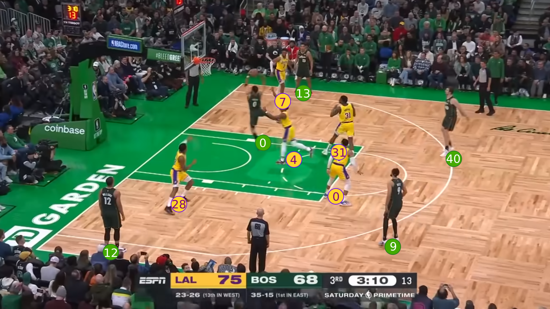
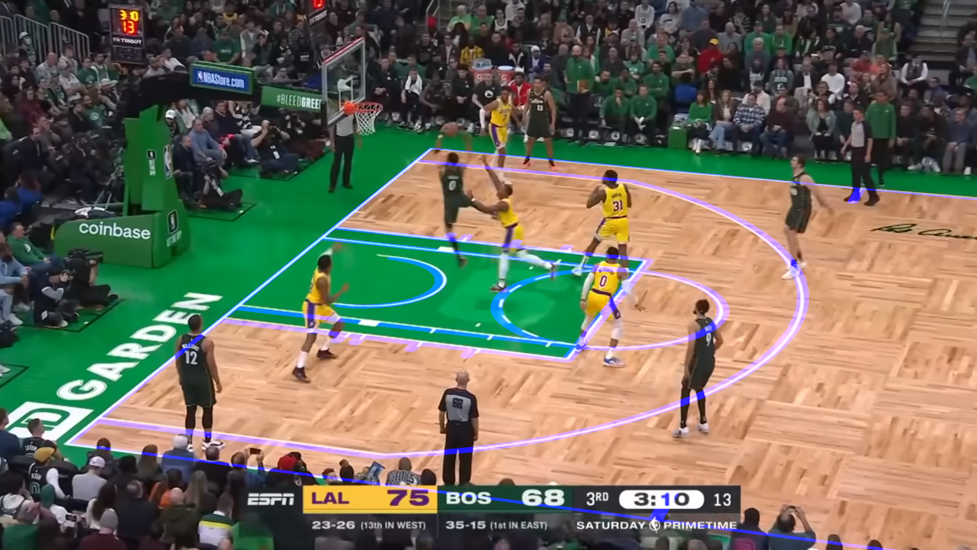
If we were able to retrieve the homography for this particular frame and locate the players on it, then we would be able to back project them and obtain their precise coordinates in the court template:

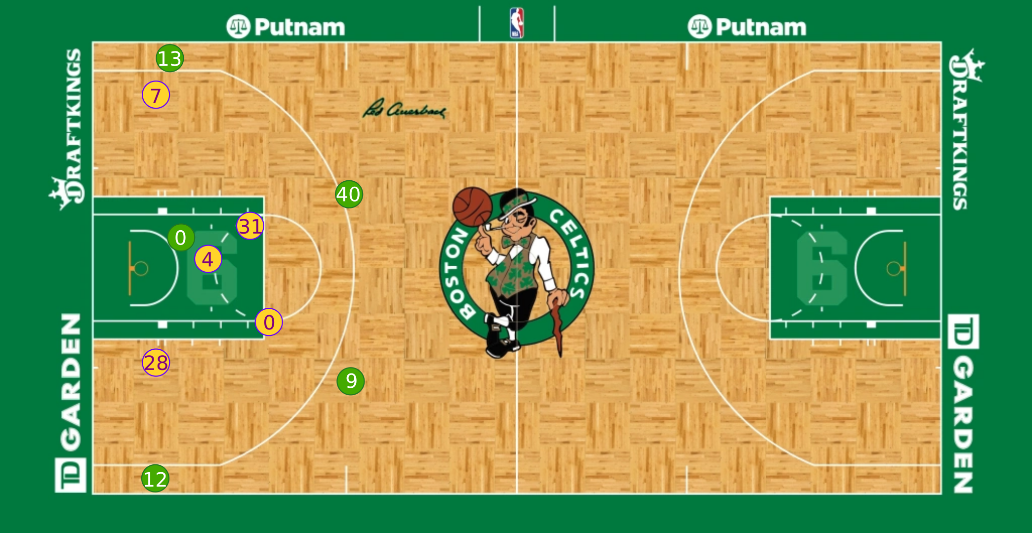
Furthermore, if we were able to do this process over all frames in the video, we would be able to track players throughout the whole game and measure any physical metric we care about.

Auxiliary repository

2. Points

In the previous post (Building the Homography Matrix from scratch), we already saw how to project a point from the 3D world into a 2D image

$$ \begin{equation} s\cdot \begin{bmatrix} x’ \\ y’ \\ 1 \\ \end{bmatrix}= \begin{bmatrix} h_{11} & h_{12} & h_{13} & h_{14}\\ h_{21} & h_{22} & h_{23} & h_{24}\\ h_{31} & h_{32} & h_{33} & h_{34}\\ \end{bmatrix} \cdot \begin{bmatrix} x \\ y \\ z \\ 1 \\ \end{bmatrix} \end{equation} $$

Importantly, this projection is not revertible. The reason is that each point in the 2D image is the result of collapsing a ray of points in the 3D world onto the image. In order to resolve the ambiguity of which one we are observing, multiple camera angles would be needed

Nevertheless, if we assume all objects of interest are located in a 2D plane, we end up with a 2D→2D mapping, which is revertible. In the scenario that motivated this post, that 2D plane in the 3D world would be the ground ($z=0$): we are interested in tracking player locations across the court, so it suffices to track their feet under the assumption that most of the time those are in the ground.

Under this circumstances, our projection simplifies to

$$ \begin{equation} s\cdot \begin{bmatrix} x’ \\ y’ \\ 1 \\ \end{bmatrix}= \begin{bmatrix} h_{11} & h_{12} & h_{13} & h_{14}\\ h_{21} & h_{22} & h_{23} & h_{24}\\ h_{31} & h_{32} & h_{33} & h_{34}\\ \end{bmatrix} \cdot \begin{bmatrix} x \\ y \\ 0 \\ 1 \\ \end{bmatrix} \end{equation} $$

or equivalently

$$ \begin{equation} s\cdot \begin{bmatrix} x’ \\ y’ \\ 1 \\ \end{bmatrix}= \begin{bmatrix} h_{11} & h_{12} & h_{14}\\ h_{21} & h_{22} & h_{24}\\ h_{31} & h_{32} & h_{34}\\ \end{bmatrix} \cdot \begin{bmatrix} x \\ y \\ 1 \\ \end{bmatrix} \end{equation} $$

So in order to project a point, we just need to convert it to homogenous coordinates and multiply with the homography matrix:

$$ \begin{equation} \vec{p’}=H\cdot\vec{p} \end{equation} $$

This will give us the projected point in homogenous coordinates. In order to retrieve the pixel location within the image, we just need to divide by the scaling factor ($s$):

$$ \begin{equation} \vec{p’}=s\cdot \begin{bmatrix} x’ \\ y’ \\ 1 \\ \end{bmatrix}\Longrightarrow x’=\frac{\vec{P}[0]}{\vec{P}[2]}, \:\:\: y’=\frac{\vec{P}[1]}{\vec{P}[2]} \end{equation} $$

Example

camera = Camera(H=np.array([
    [ 8.69135802e+00, -2.96296296e+00,  6.40000000e+02], 
    [ 0.00000000e+00,  7.33333333e+00,  2.93333333e+02], 
    [ 0.00000000e+00, -4.62962963e-03,  1.00000000e+00],
]))

pt = Point(x=0, y=0)

projected_pt = project_points(camera=camera, pts=(pt, ))

print(projected_pt[0])

>>> Point(x=640.0, y=293.333333)

3. Lines

A straight line is fully described in 2D through its vector representation $\vec{l}$

$$ \begin{equation} \vec{l}= \begin{bmatrix} a \\ b \\ c \\ \end{bmatrix} \end{equation} $$

A point expressed in homogeneous coordinates, $\vec{p}=[x, y]^T$, belongs to the line if it satisfies its general form

$$ \begin{equation} a\cdot x + b\cdot y + c = 0 \end{equation} $$

That is to say, it is orthogonal to the line vector

$$ \begin{equation} \vec{l}^T\cdot \vec{p} = 0 \end{equation} $$

We can leverage the basic property of collinearity preservation under projective geometry: if a point $\vec{p}$ lies in a line $\vec{l}$, the projected point $\vec{p’}=H\cdot\vec{p}$ will lie in the projected line $\vec{l’}$. Therefore, it must satisfy

$$ \begin{equation} \vec{l’}^T\cdot \vec{p’} = 0 \end{equation} $$

or equivalently

$$ \begin{equation} \vec{l’}^T\cdot H \cdot \vec{p} = 0 \end{equation} $$

Since both equations are null, they must be equal

$$ \begin{equation} \vec{l}^T\cdot\vec{p’} = \vec{l’}^T\cdot H\cdot\vec{p} \end{equation} $$

which necessarily implies

$$ \begin{equation} \vec{l}^T = \vec{l’}^T\cdot H \end{equation} $$

Consequently, in order to project a line, we simply need to apply

$$ \begin{equation} \vec{l’} = H^{-T}\cdot \vec{l} \end{equation} $$

Example

camera = Camera(H=np.array([
    [ 8.69135802e+00, -2.96296296e+00,  6.40000000e+02], 
    [ 0.00000000e+00,  7.33333333e+00,  2.93333333e+02], 
    [ 0.00000000e+00, -4.62962963e-03,  1.00000000e+00],
]))

ln = Line(a=0, b=1, c=0)

projected_ln = project_lines(camera=camera, lines=(ln, ))

print(projected_ln[0])

>>> Line(a=0.0, b=7.33333333, c=293.333333)

4. Conics

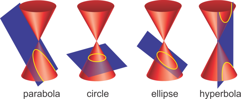
Conic curves receive their name since they can be obtained fr the intersection between a plane and a cone with two nappes:

• Circle: plane is perpendicular to the cone axis
• Ellipse: plane intersects with only one half of the plane forming a closed surface
• Hyperbola: plane intersects with both halves of the plane
• Parabola: plane is parallel to the cone slant

4.1. Projection

Mathematically, a conic curve can be modelled by means of its matrix representation $M$:

$$ \begin{equation} M= \begin{bmatrix} A & B/2 & D/2 \\ B/2 & C & E/2 \\ D/2 & E/2 & F \\ \end{bmatrix} \end{equation} $$

Any point that belongs to it, expressed in homogeneous coordinates, $\vec{p}=[x, y, 1]^T$, must satisfy the following second-degree polynomial equation:

$$ \begin{equation} A\cdot x^2 + B\cdot x\cdot y + C\cdot y^2 + D \cdot x + E \cdot y + F = 0 \end{equation} $$

or in matrix form:

$$ \begin{equation} \vec{p}^T\cdot M \cdot \vec{p} = 0 \end{equation} $$

Once again, we can take advantage of the collinearity preservation property, which is valid for any kind of line, not just straight one. Let us say that a point $\vec{p}$ lies in the ellipse given by $M$. Then the projected point $\vec{p’}=H\cdot\vec{p}$ must lie in the projected ellipse given by $M'$

$$ \begin{equation} \vec{p’}^T\cdot M’ \cdot \vec{p’} = 0 \end{equation} $$

Replacing the projected point we obtain

$$ \begin{equation} (H\cdot\vec{p})^T\cdot M’ \cdot H\cdot\vec{p} = 0 \end{equation} $$

Notice the equivalence of the previous null equations

$$ \begin{equation} \vec{p}^T\cdot H^T\cdot M’ \cdot H\cdot\vec{p} = \vec{p}^T\cdot M \cdot \vec{p} \end{equation} $$

which necessarily implies

$$ \begin{equation} H^T\cdot M’ \cdot H = M \end{equation} $$

Therefore, projecting a conic reduces to

$$ \begin{equation} M’ = H^{-T}\cdot M \cdot H^{-1} \end{equation} $$

4.2. Distortion: Objects behind the camera plane

Importantly, although the projective transform maps a conic to another conic, it does not necessarily preserve its type. It is not hard to visualise how a circle can become an ellipse depending on the perspective. However, it is not intuitive at all how it might turn into a parabola/hyperbola. So what is going on?

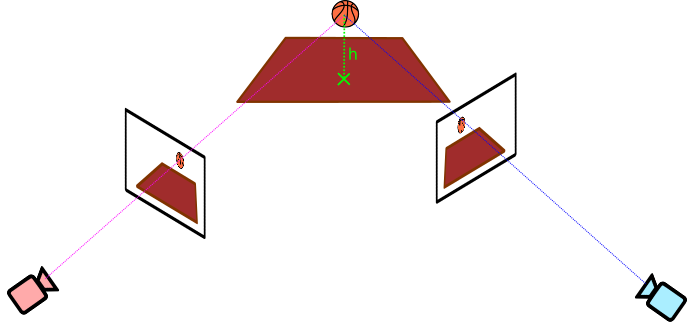
The key feature is the camera plane. It corresponds to the 2D plane parallel to the camera film (where the image is projected onto) that passes through the camera pinhole. Objects in front of it are projected to the film plane (the infinite extension of the film with finite dimensions), but are only captured in the image whenever they lie within the covered pyramid, as displayed below:

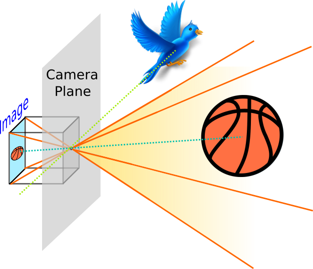
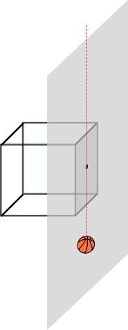
On the other hands, objects that lie right on the camera plane would never be projected onto the image plane, since the ray that goes both through them and the pinhole is parallel to the image plane:

Finally, when an object is behind the camera plane, the projective transform is still able to project it onto the image film.

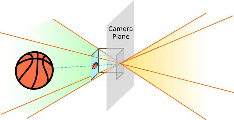
However, this is a mathematical artefact!!! Whenever we take a picture, we ca only capture objects within the field of view in front of the camera. Nonetheless, the mathematical transform that models this process can still be applied to objects behind the camera. Therefore, one must be careful and ensure this transform is restricted to objects in front of the camera, or we’d introduced unexpected distortions.

Let us now go back to the case of conics. In order to better gain some insight, let us picture the following scenario: a couple of friends are playing frisbee and there happens to be a drone recording the scene from above

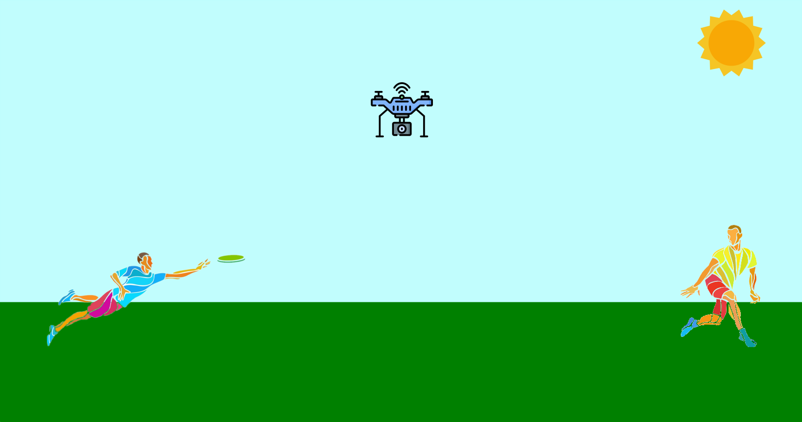
To further simplify the scenario, let us assume the frisbee, of radius $r$, is the only object the camera is able to track. Furthermore, it is following a perfectly horizontal and straight trajectory in a plane parallel to the camera axis, starting at a distance $d$. The camera has focal length $f$ and projects onto an image of size $(W, H)$. Finally, let us define the origin of coordinates in our 3D world at the intersection between the 2D plane the frisbee travels through and the vertical line passing through the camera pinhole, located at a height $h$.

The following video displays what we would get if we were to mathematically compute the projection of the conic and display it on the image film. For clarity, we provide at the bottom an amplified view of the virtual image (the result of flipping horizontally and vertically the film image):

Whenever the frisbee is right at the edge of the camera plane, the frisbee gets mapped to a parabola. The reason is that point at the edge gets mapped to infinity, turning the circular frisbee into an open surface.

Moreover, whenever the frisbee is partially in front of the camera, and partially behind it, there is a split in the projection. As a result, we get the unexpected hyperbola. Again, this is a mathematical artefact that would never manifest in a real photograph, it only arises if one naively projects without considering the location of objects w.r.t. the camera plane.

Note: you can generate the previous video by simply running this script. In order to do so, just install the repository (poetry install) and then run

poetry run python -m projective_geometry frisbee-demo --output <LOCATION_OUTPUT_VIDEO.mp4>

5. Images

In order to project an image, we start by building a $(3, N)$ matrix $P=[\vec{X}\,\,\,\vec{Y} \,\,\,\vec{1} ]^T$ with the homogenous coordinates for all pixels in the image grid:

Then we project the grid of points using the homography matrix characterising the camera and convert the resulting homogeneous coordinates to pixel locations

$$ \begin{equation} P’ = H\cdot P \end{equation} $$

$$ \begin{equation} p_i’’=\left[\frac{p_i’[0]}{p_i’[2]}, \frac{p_i’[1]}{p_i’[2]}\right] \,\,\,\,\,\,\,\,\forall p_i’\in P' \end{equation} $$

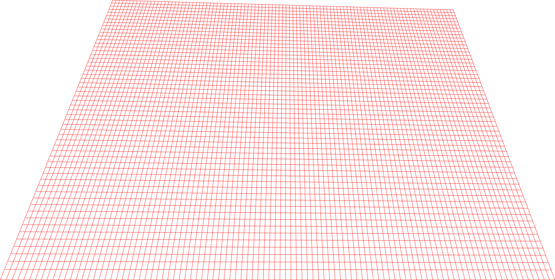
Finally, we just need to interpolate the image values at the projected grid

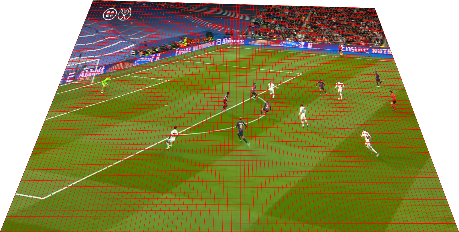
OpenCV provides a method that applies this transform, cv2.warpPerspective. It provides different methods to carry out the interpolation, some of which are differentiable. Differentiability becomes essential for dealing with optimization problems. Most often, this kind of problems are tackled via gradient-descent algorithms. Therefore, whenever the image projection transform is part of the cost function we are trying to optimize for, one must ensure the underlying interpolation is carried out in a differentiable fashion.

This is useful for validating if a camera is properly corrected by visual inspection. You can simply project the source image using the camera and validate it overlaps with the target image. There is an example in case you want to try it out by yourself here, which you can run with the command below

poetry run python -m projective_geometry celtics-demo --output <LOCATION_OUTPUT_IMAGE.png>

This will display the projected court template on top of the given frame

5.1. Projection via object decomposition

Notice that when projecting a line, its width varies depending on where it lands on the image. This is expected behaviour and reflects how we perceive the 3D world: objects closer to us occupy a wider field of view than those further away.

However, in some scenarios, one might be interested in having full control over the visualisation of projected objects. Whenever it is feasible to decompose the original image in its core geometric features, one could therefore project individually each feature and display it on the target image with the desired visualisation properties. For instance, the basketball court ban be broken down into all the line segments, circles and arcs, as illustrated below

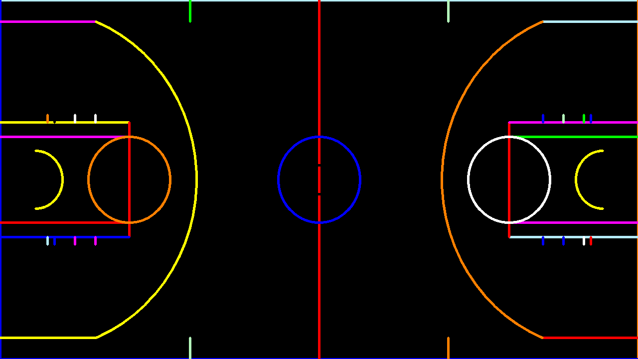
The drawback, as already explained, is that objects might be partially or completely behind the camera plane. Consequently, if following this approach, it is essential to exclude those objects from the visualisation in order to avoid undesired artefacts.

6. References

1. Richard Hartley and Andrew Zisserman (2000), Page 143, Multiple View Geometry in Computer Vision, Cambridge University Press.
2. Wikipedia. Conic sections and Matrix Representation
3. Wei Jiang et. al. (2019), arXiv. Optimizing Through Learned Errors for Accurate Sports Field Registration
4. OpenCV Library