Table of Contents
1. Introduction
In the last post we saw how to retrieve the 3D location of a ball from its 2D image projection, represented as an ellipse. However, this approach is quite prone to noise since it only uses a single frame.
A more robust method would involve having multiple frames of the ball in motion and fitting a physically plausible trajectory to the observed projections. In this post, we will explore how to model the 3D trajectory of a ball under various physical effects and how to estimate this trajectory from its 2D projections.
 Auxiliary repository
2. Simulating a 3D ball trajectory
The goal of this section is to characterize the equations of motion of a ball under different physical effects it undergoes. To do so, we will define a vector $\mathbf{s}(t)$ that captures the state of the ball at any given time $t$. We will then define a differential equation that describes how this state changes over time:
$$ \begin{equation} \frac{d\mathbf{s}(t)}{dt} = f(\mathbf{s}(t), t) \end{equation} $$
where $f$ is a function that encapsulates the physical effects acting on the ball. By integrating this differential equation over time, we can obtain the trajectory of the ball. This integration can be performed numerically using methods such as Euler’s method or the Runge-Kutta method. In particular, we will leverage the ‘solve_ivp’ function from the SciPy library to perform this integration.
Solving the differential equation will give us the 3D position of the ball at any time $t$. In order to simulate what we capture through a camera, we will also need to project this 3D position onto the 2D image plane using the camera projection matrix $\mathbf{P}$, as we did in the previous post.
Let us see what these effects are and how they affect the ball’s trajectory.
2.1. Gravity
Any object experiences the force of gravity pulling it downwards. We can define a state vector for the ball that comprises its position $\mathbf{p}(t)$ and velocity $\mathbf{v}(t)$ in 3D space:
$$ \begin{equation} \mathbf{s}(t) = \begin{bmatrix} \mathbf{p}(t), \ \mathbf{v}(t) \end{bmatrix} \end{equation} $$
Gravity acts in the negative z-direction, causing a constant downwards acceleration given by:
$$ \begin{equation} \mathbf{a}_g = \begin{bmatrix} 0 \ 0 \ -10.72 \end{bmatrix} \text{ yds/s}^2 \end{equation} $$
Since acceleration is the derivative of velocity, we can express the equations of motion as follows:
$$ \begin{equation} \frac{d\mathbf{s}(t)}{dt} = \begin{bmatrix} \mathbf{v}(t), \ \mathbf{a}_g(t) \end{bmatrix} \end{equation} $$
Given some initial conditions $\mathbf{p}(0) = \mathbf{p}_0$ and $\mathbf{v}(0) = \mathbf{v}_0$, we can integrate these equations over time to obtain the ball’s trajectory.
We will illustrate the ball trajectories under the influence of the different physical effects we introduce via interactive visualizations. In the one below, we display a goal kick. You can modify the initial position of the ball in the small box on the left (y0) and the time (t) to see how the ball moves in 3D space and how its projection (ellipse) changes in the image.
Goal kick captured from broadcast angle
XY projection of goal kick from bird's eye view
2.2. Bouncing
Look carefully at the previous visualization. We set up the simulation to prevent the ball from going below ground level. To do so we simply detected when the ball hit the ground ($z=0$) going downwards ($vz<0$) and fixed its position wherever it landed for the rest of the simulation. However, in reality, the ball bounces when it hits the ground.
To model the bouncing effect, we need to consider the coefficient of restitution (COR), which quantifies how much kinetic energy is conserved during a collision. A COR of 1 means a perfectly elastic collision (no energy loss), while a COR of 0 means a perfectly inelastic collision (the ball does not bounce at all).
When the ball hits the ground (z=0), we reverse its vertical velocity component and scale it by the COR:
$$ \begin{equation} v_z’ = -\text{COR} \cdot v_z \end{equation} $$
Therefore, to simulate bouncing, we need to:
- Detect a collision with the ground
- Manually update the vertical velocity component according to the COR
- Restart the simulation from the new state after the bounce
In the following interactive visualization, you can modify the initial velocity magnitude (|v|) and the time (t) to see how the ball moves in 3D space. Notice how the ball bounces when it hits the ground.
Goal kick captured from broadcast angle
XY projection of goal kick from bird's eye view
2.3. Friction and drag
Another caveat of the previous simulations is that the ball maintains its horizontal velocity indefinitely. In reality, the ball experiences friction and air resistance (drag) that slow it down over time. To model these effects, we can introduce two additional forces:
Friction: When the ball is in contact with the ground, it experiences a frictional force that opposes its horizontal motion. This force is proportional to the normal force (weight of the ball) and a coefficient of friction $\mu$. The frictional acceleration acts in the opposite direction of the horizontal velocity and can be expressed as:
$$ \begin{equation} \mathbf{a}_f = -\mu g |\mathbf{u}_h \end{equation} $$
where $\mathbf{v}_h = [v_x, v_y]$ is the horizontal component of the velocity, $\mathbf{u}_h$ is the unit vector in the direction of $\mathbf{v}_h$ and $g$ is the gravitational acceleration magnitude.
Drag: Air resistance creates a drag force that opposes the ball’s motion in all directions. This force follows the quadratic drag equation:
$$ \begin{equation} F_d = \frac{1}{2} \rho |\mathbf{v}|^2 C_d A \end{equation} $$
where $\rho$ is air density, $v$ is the speed, $C_d$ is the drag coefficient, and $A$ is the cross-sectional area. Converting this to acceleration by dividing by the ball mass $m$, and applying it in the direction opposite to velocity:
$$ \begin{equation} \mathbf{a}_d= -\frac{\rho C_d A}{2m} |\mathbf{v}|^2 \mathbf{u}_v \end{equation} $$
where $\mathbf{u}_v = \frac{\mathbf{v}}{|\mathbf{v}|}$ is the unit vector in the direction of velocity.
The total acceleration is now the sum of gravity, friction (when on the ground), and drag. Thus our equations of motion become:
$$ \begin{equation} \frac{d\mathbf{s}(t)}{dt} = \begin{bmatrix} \mathbf{v}(t), \ \mathbf{a}_g(t)+ \mathbf{a}_f(t) + \mathbf{a}_d(t) \end{bmatrix} \end{equation} $$
In the visualization below, you can observe how these forces cause the ball to slow down both horizontally and vertically. The angle slider ($\measuredangle_v$) controls the initial angle of the velocity vector with respect to the ground. Note that friction only acts when the ball is in contact with the ground.
Goal kick captured from broadcast angle
XY projection of goal kick from bird's eye view
2.4. Magnus effect
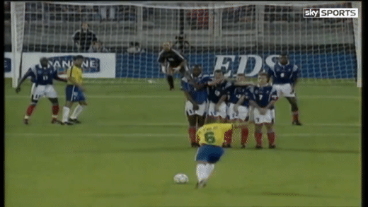
Roberto Carlos scored one of the most famous free kicks in football history during the 1997 Tournoi de France against France, knwon as the ‘banana kick’:
Now, think for a moment: do you think our current model can explain such a curved trajectory? The answer is no. Notice how the XY projection of the ball’s trajectory in the previous visualizations is always a straight line.
To model such curved trajectories, we need to introduce the Magnus effect, which occurs when a spinning ball moves through the air. The spin creates a pressure differential around the ball, resulting in a lift force that acts perpendicular to the direction of motion and the axis of rotation. You can find a great explainer about the Magnus effect in this YouTube video.
This implies that we need to extend our state vector to include the ball’s angular velocity $\boldsymbol{\omega}(t)$:
$$ \begin{equation} \mathbf{s}(t) = \begin{bmatrix} \mathbf{p}(t), \ \mathbf{v}(t), \ \boldsymbol{\omega}(t) \end{bmatrix} \end{equation} $$
The Magnus acceleration can be expressed as:
$$ \begin{equation} \mathbf{a}_m = \frac{\rho A C_L}{2m} (\boldsymbol{\omega} \times \mathbf{v}) \end{equation} $$
where $C_L$ is the Magnus lift coefficient, and the cross product $\boldsymbol{\omega} \times \mathbf{v}$ gives the direction of the Magnus force perpendicular to both the spin axis and velocity.
Thus, our equations of motion now become:
$$ \begin{equation} \frac{d\mathbf{s}(t)}{dt} = \begin{bmatrix} \mathbf{v}(t), \ \mathbf{a}_g(t)+ \mathbf{a}_f(t) + \mathbf{a}_d(t) + \mathbf{a}_m(t), \ \mathbf{0} \end{bmatrix} \end{equation} $$
We could also model the decay of angular velocity over time due to air resistance, but for simplicity, we will assume it remains constant in this simulation.
In the following interactive visualization, you can modify the initial angular velocity around the z-axis ($\omega_{z0}$) and the time (t) to see how the ball moves in 3D space. Notice how the Magnus effect causes the ball to curve in flight.
Goal kick captured from broadcast angle
XY projection of goal kick from bird's eye view
2.5. Putting it all together
We now have all the ingredients we need. But let us add a final pinch of salt: measurement noise. We will add two sources of noise to our simulation:
- Positional noise: We will add Gaussian noise with standard deviation $\sigma_N$ to the 2D projected position of the ball in the image plane. This simulates inaccuracies in detecting the ball’s position in the image.
- Missed detections: We will randomly drop some frames with a probability $P_M$ to simulate missed detections, which are common in real-world scenarios due to occlusions, motion blur or simply failing to detect the ball.
Goal kick captured from broadcast angle
XY projection of goal kick from bird's eye view
You can find the complete code for the simulation engine here.
3. Estimating the 3D ball trajectory
We have now built a simulation engine that maps an initial state $\mathbf{s}_0=\begin{bmatrix} \mathbf{p}_0, \mathbf{v}_0, \boldsymbol{\omega}_0 \end{bmatrix}$ to a temporal sequence of 2D objects $O_i=O(t_i)$ representing the ball projections in the image plane at different time steps $t_i$.
Our goal now is to invert this process: given a set of observed 2D objects $O’_i$ at times $t_i$, can we retrieve the initial state $\mathbf{s}_0$ that best explains these observations?
In order to do so we need to define two components:
- A cost function that quantifies how well a given initial state $\mathbf{s}_0$ explains the observed 2D objects $O’_i$.
- An optimization algorithm that searches for the initial state $\mathbf{s}_0$ that globally minimizes this cost function.
3.1. Cost function
The cost function $\mathcal{C}(s_0)$ measures the discrepancy between the observed 2D objects $O’_i$ and the projected 2D objects $O_i$ generated by simulating the ball trajectory from a given initial state $\mathbf{s}_0$:
$$ \begin{equation} \mathcal{C}(s_0) = \sum_{i} e_i(O’_i, O_i(s_0)) \end{equation} $$
where $e_i$ is an error metric that quantifies the error between the observed object $O’_i$ and the projected object $O_i(s_0)$ at time $t_i$. Depending on how we represent the 2D objects, we can define different types of cost functions. You can find their implementations here.
3.1.1. Ellipse fitting
Up to now, our visualizations have represented the ball projections as ellipses. Therefore we need a metric that quantifies the error between two ellipses. Below you can see an example of the observed ellipses (ellipse outlines marked in red) for a pass in a basketball game:
Pass captured from broadcast angle
XY projection of pass from bird's eye view
One may naively think of measuring the distance between the ellipse parameters (center, axes, orientation). However, this approach is not robust due to the ambiguities in ellipse parameterization. For instance, the same ellipse can be represented with swapped axes and a 90-degree rotation.
One way to circumvent this issue is by sampling $N$ points $\{ p’_{ij} \} _{j=1}^{N}$ along the observed ellipse $O_i’$ and measuring their distance to the estimated ellipse $O_i(s_0)$. Thus, we can define the error metric as the sum of distances from the sampled points to the estimated ellipse:
$$ \begin{equation} e_i(O_i’, O_i(s_0)) = \sum_{j=1}^{N} d(p’_{ij}, O_i(s_0)) \end{equation} $$
We will now explore two different distance metrics $d(p, O)$ that can be used in this context.
3.1.1.1. Algebraic distance
An ellipse in 2D can be parametrized by its matrix representation $\mathbf{C}$. Any point $\mathbf{p}=[x, y, 1]^T$ lying on the ellipse satisfies the following equation:
$$ \begin{equation} \mathbf{p}^T \mathbf{C} \mathbf{p} = 0 \end{equation} $$
We can extend this equation and define the function:
$$ \begin{equation} f(\mathbf{x, y}) = \mathbf{p}^T \mathbf{C} \mathbf{p} \end{equation} $$
This function defines a paraboloid surface where the ellipse corresponds to the zero level set. The figure below shows a 3D visualization of this paraboloid surface for a given ellipse:
Furthermore, its isocontours given by $f(\mathbf{x, y}) = k$ represent scaled versions of the ellipse. The figure below illustrates these isocontours for different values of $k$:
Based on this observation, we can define the algebraic distance from a point $\mathbf{p}$ to the ellipse represented by matrix $\mathbf{C}$ as:
$$ \begin{equation} d_{\text{alg}}(\mathbf{p}, \mathbf{C}) = |\mathbf{p}^T \mathbf{C} \mathbf{p}| \end{equation} $$
This distance measures how far the point is from lying on the ellipse in terms of the paraboloid function value. In other words, it captures what isocontour the point lies on. The bigger the value, the further the isocontour from the ellipse.
3.1.1.2. Sampson distance
One limitation of the algebraic distance is that it does not correspond to a geometric distance in the image plane. Ideally, we would like to measure the shortest Euclidean distance from the point to the ellipse.
$$ \begin{equation} d_{\text{geo}}(\mathbf{p}, \mathbf{C}) = \min_{\mathbf{q} \in \text{ellipse}} || \mathbf{p} - \mathbf{q} || \end{equation} $$
However, computing this geometric distance is not straightforward, as it involves solving a quartic equation. Instead, we can use the Sampson distance, which provides a first-order approximation of the geometric distance. The Sampson distance is defined as:
$$ \begin{equation} d_{\text{Sampson}}(\mathbf{p}, \mathbf{C}) = \frac{(\mathbf{p}^T \mathbf{C} \mathbf{p})^2}{(2 \mathbf{C} \mathbf{p})_x^2 + (2 \mathbf{C} \mathbf{p})_y^2} \end{equation} $$
We provide a detailed derivation of this formula for the interested reader below:
Sampson distance derivation
Given a noisy measurement vector $\mathbf{p} \in \mathbb{R}^n$ and a constraint function $f(\mathbf{p}) \in \mathbb{R}^m$, the goal is to find a corrected vector $\mathbf{p} + \delta \mathbf{p}$ that lies on the manifold defined by $f(\mathbf{p}) = 0$, while minimizing the correction magnitude $|| \delta \mathbf{p} ||^2$: $$ \begin{equation} \delta \mathbf{p} = \arg \min_{\delta \mathbf{p}} || \delta \mathbf{p} ||^2 \quad \text{s.t.} \quad f(\mathbf{p} + \delta \mathbf{p}) = 0 \end{equation} $$ This is illustrated below for the case of an ellipse constraint $f(\mathbf{p}) = p_H^T\cdot C\cdot p_H=0$:3.1.2. Bounding box fitting
In many practical scenarios, the ball detections are represented as bounding boxes rather than ellipses. This is the case when using object detection models like YOLO or Faster R-CNN, which output axis-aligned bounding boxes around detected objects.
Our simiulation engine produces ellipses, so we need an additional step to convert these ellipses into bounding boxes. To do so, recall an ellipse with parameters centered at $(0, 0)$, with semi-major axis $a$, semi-minor axis $b$, and orientation angle $\theta$ can be parametrized as:
$$ \begin{equation} \frac{(x \cos \theta - y \sin \theta)^2}{a^2} + \frac{(x \sin \theta + y \cos \theta)^2}{b^2} = 1 \end{equation} $$
The derivative is given by:
$$ \begin{equation} \frac{d y}{d x} = -\frac{a^2 x \sin^2\theta + y(a-b)(a+b)\sin\theta\cos\theta + b^2 x \cos^2\theta}{a^2 y \cos^2\theta + x(a-b)(a+b)\sin\theta\cos\theta + b^2 y \sin^2\theta} \end{equation} $$
We are looking for the points where the tangent is vertical or horizontal, i.e. where $\frac{d y}{d x} = 0$ or $\frac{d x}{d y} = 0$. Carefully solving these equations and shifting to allow for ellipses not centered at the origin, we obtain the following four points:
$$ \begin{equation} \begin{aligned} x = x_0 \pm \sqrt{a^2\cos^2\theta + b^2\sin^2\theta} \\ y = y_0 \pm \sqrt{a^2\sin^2\theta + b^2\cos^2\theta} \end{aligned} \end{equation} $$
Below you can see an example of the observed bounding boxes (outlined in red) for a pass in a basketball game:
Pass captured from broadcast angle
XY projection of pass from bird's eye view
We can encode the bounding box as the coordinates of the top-left and bottom-right corners: $O_i = [\mathrm{t}_l, \mathrm{b}_r] = [t^x_l, t^y_l, b^x_r, b^y_r]$. A couple choices for the error metric $e_i$ between the observed bounding box $O’_i$ and the projected bounding box $O_i(s_0)$ are given below.
3.1.2.1. L2 distance
One option is to simply measure the L2 distance between the top-left and bottom-right corners of the bounding boxes: $$ \begin{equation} \begin{aligned} e_i(O_i’, O_i(s_0)) & = || O_i’ - O_i(s_0) ||^2 \\ &= || t’_l - t_l(s_0) ||^2 + || b’_r - b_r(s_0) ||^2 \end{aligned} \end{equation} $$
3.1.2.2. YOLO loss
While the L2 distance is simple and straightforward, it has some limitations. For instance, it treats all pixels equally, even though errors in the width and height might be more or less important than errors in position.
The YOLO (You Only Look Once) object detection framework encodes the bbox as $O=(c, a)$, where $c=(x_c, y_c)$ is the bbox center and $a=(w, h)$ is the size (width and height). The YOLO loss function combines errors in both center position and size, with different weighting factors:
$$ \begin{equation} e_i(O_i’, O_i(s_0)) = \lambda_c \cdot e_i^c(c’, c_i(s_0)) + \lambda_s \cdot e_i^s(a_i’, a_i(s_0)) \end{equation} $$
where $\lambda_c$ and $\lambda_s$ are weighting factors that control the importance of the corresponding terms given by:
$$ \begin{equation} e_i^c(c’, c_i(s_0)) = || c’ - c_i(s_0) ||^2 \end{equation} $$
and
$$ \begin{equation} e_i^s(a’, a_i(s_0)) = || \sqrt{w’} - \sqrt{w_i(s_0)} ||^2 + || \sqrt{h’} - \sqrt{h_i(s_0)} ||^2 \end{equation} $$
The key innovation here is the use of square roots for the width and height terms, which penalizes errors in small boxes more than in large boxes.
3.2. Optimization
Now that we have defined cost functions to measure the quality of a trajectory estimate, we need an optimization algorithm to find the initial state $\mathbf{s}_0 = [\mathbf{p}_0, \mathbf{v}_0, \boldsymbol{\omega}_0]$ that minimizes this cost.
Our goal is to find the global minimum of the cost function. However, this is challenging because the cost function is non-convex, meaning it has multiple local minima. The main source of non-convexity is the bouncing in the trajectory—the abrupt changes in velocity when the ball hits the ground create discontinuities that lead to multiple local minima in the optimization landscape.
There are two sensible approaches to overcome this challenge:
-
Partial trajectory fitting: Identify the bouncing points and break the problem into fitting the trajectory per segments in between bounces. The final state of each segment serves as the initial state for the next segment. In this scenario, the optimization becomes locally convex within each segment, making gradient-based methods well-suited for the task. Common choices include Gradient Descent, Levenberg-Marquardt, and L-BFGS-B.
-
Global optimization methods: Use gradient-free methods that can explore different regions of the parameter space in search of the global minimum, thus avoiding getting stuck in local minima. Common choices include Nelder-Mead Simplex and Differential Evolution.
Picking a good initial guess for the parameters is crucial for the success of both approaches. To do so, one can estimate the initial trajectory frame-wise with the method described in our previous post and then infer the initial state $\mathbf{s}_0$ from these estimates.
4. Demo
You can find an implementation of these optimization methods in the auxiliary GitHub repository. We provide an example that you can try yourself by running this script:
poetry run python -m projective_geometry locate-3d-ball-trajectory-demo
It will generate the ball trajectory displayed below (gray) and corrupt the observations (red) with noise and missed detections:
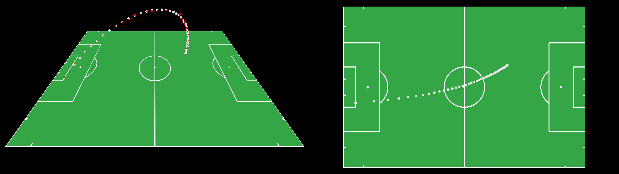
Then it will plot the estimated trajectory (blue) against the ground-truth (gray):
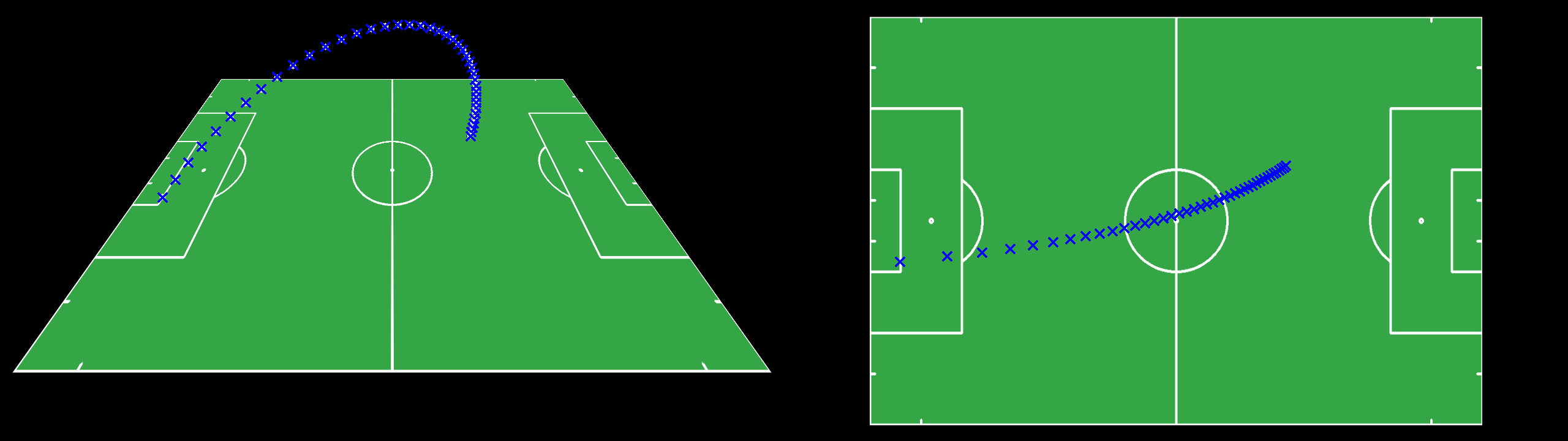
It uses the algebraic distance by default, but you can easily switch to any of the other cost functions described above by passing the corresponding argument to the entrypoint function. It also uses a convex optimizer (L-BFGS-B) by default, but you can switch to a global optimizer (Differential Evolution) as well, which is particularly useful when there is bouncing in the trajectory.
5. Conclusion
In this post, we have explored how to estimate the 3D trajectory of a ball from its 2D projections in video frames. We started by building a comprehensive physics simulation that models the ball’s motion under various forces:
- Gravity: The fundamental force pulling the ball downward
- Bouncing: Modeled using the coefficient of restitution to simulate energy loss during collisions
- Friction and drag: Air resistance and ground friction that slow the ball down
- Magnus effect: The force resulting from ball spin that creates curved trajectories
By formulating these effects as a system of differential equations, we created a forward model that maps an initial state $\mathbf{s}_0 = [\mathbf{p}_0, \mathbf{v}_0, \boldsymbol{\omega}_0]$ to a temporal sequence of 2D projections.
Then we focused on the inverse problem: estimating the initial state from observed 2D projections. We framed it as a non-linear optimization problem and explored different cost functions based on:
- Ellipse fitting: Using algebraic distance or Sampson distance to measure discrepancy between observed and predicted ellipses
- Bounding box fitting: Using L2 distance or YOLO-style loss for axis-aligned bounding boxes
We have also provided interactive visualizations to illustrate the concepts discussed, as well as an auxiliary repository with the complete code implementation.
6. References
- Richard Hartley and Andrew Zisserman (2000), Page 143, Multiple View Geometry in Computer Vision, Cambridge University Press.
- SciPy. Optimize module
- Math Stack Exchabge. How to get the limits of rotated ellipse
- Spiff. Magnus effect
7.Clarify
Given a noisy measurement vector $\mathbf{p} \in \mathbb{R}^n$ and a constraint function $f(\mathbf{p}) \in \mathbb{R}^m$, the goal is to find a corrected vector $\mathbf{p} + \delta \mathbf{p}$ that lies on the manifold defined by $f(\mathbf{p}) = 0$, while minimizing the correction magnitude $|| \delta \mathbf{p} ||^2$: $$ \begin{equation} \delta \mathbf{p} = \arg \min_{\delta \mathbf{p}} || \delta \mathbf{p} ||^2 \quad \text{s.t.} \quad f(\mathbf{p} + \delta \mathbf{p}) = 0 \end{equation} $$ This is illustrated below for the case of an ellipse constraint $f(\mathbf{p}) = p_H^T\cdot C\cdot p_H=0$: