Table of Contents
In this article we will focus on the topic of Compressed Sensing. We will start by motivating the interest in this recent field. Sparse signals are ubiquitous in nature, and the ability to recover them from a small number of measurements has a wide range of applications. We will try and understand the mathematical underpinnings of the theory, and why the l1-norm is used as a proxy for sparsity.
1. Data compression
In recent times, the amount of data generated each day is staggering, and it is only increasing. We deal with vasts amounts of data that aim at capturing some form of representation of the natural world around us. Take images for example. An image can be thought of as a $W \times H$ 2D array of pixels, where each pixel is a 3-tuple of RGB values represented with $B$ bits per channel. That means there are $2^{3 \cdot B \cdot W \cdot H}$ possible images we could have, which is a mind-boggling number. However, that begs the question: how many of these images are actually interesting?
The answer is not that many. If you were to randomly generate images, it is highly likely that you would never create one that looks like nothing more than noise, even if you spent an eternity doing so.. This is because natural images are not random, they have structure and patterns that make them interesting.

The number of natural images (and by this we mean not only images that one could observe in the real world, but also any image inspired by it that may only live in one’s imagination) is inmense. However, it is still a tiny fraction of the total number of possible images. That suggests natural images should be highly compressible. We just need to find a suitable basis to represent them in a more compact way.
The diagram above shows the standard procedure we follow to capture images. We use a device such as a camera to take a sample of the world around us. Then this sample is processed in order to compress it. Finally, the compressed data is stored in a digital format. The goal of this process is to minimize the amount of data we need to store while preserving the most important information.
2. Compressed sensing
The process described above seems inefficient at first sight. If compressing the image allows to discard a lot of redundant information and store only a small fraction of coefficients to represent it, why do we need to take so many measurements (all pixels in the image) in the first place? Can we not directly sample in a compressed way in order to speed up the process? This is the question that Compressed Sensing (also termed Compressive Sampling) tries to answer.
You might be wondering at this point though: did not the Shannon-Nyquist theorem tell us that we need to sample at a rate at least twice the highest frequency in the signal in order to be able to reconstruct it? How can one expect to sample at a rate lower than that and still be able to recover the signal?
Sampling a continuous signal leads inevitably to an ambiguity whenever one tries to retrieve the original signal from a set of discrete measurements. There are infinite ways in which one could do so. However, the key insight is that if one has additional knowledge about the signal, uniquely reconstructing it becomes possible. In the Shannon-Nyquist scenario, that knowledge is that the bandwith of the sampled signal $B$ is below half the sampling frequency $f_s$: $B \leq \frac{f_s}{2}$).
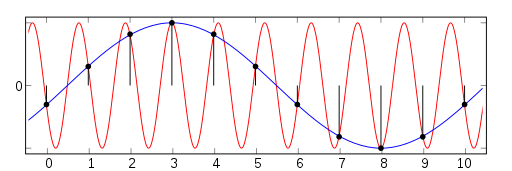
Compressed sensing is based on the same principle, but goes one step further. It assumes that the signal we are trying to recover is sparse in a suitable basis. Depending on the level of sparsity, this may end up being a much more restrictive assumption than the one made by the Shannon-Nyquist theorem. But that is exactly the reason why we may get away with taking far fewer measurements than the Nyquist rate.
2.1. Problem formulation
Compressed sensing operates on the assumption that the signal we are trying to recover $\mathbf{x} \in \mathbb{R}^N$ is $k$-sparse in a suitable basis, given by the columns of matrix $\mathbf{\Psi}$. That means $\mathbf{x}$ can be represented as:
$$ \begin{equation} \mathbf{x} = \mathbf{\Psi} \mathbf{s} \end{equation} $$
where $\mathbf{s} \in \mathbb{R}^N$ is a sparse vector, with at most $k$ non-zero entries. . We are interested in recovering $\mathbf{x}$ from a set of $M$ linear measurements, with $M < N$. The measurements $\mathbf{y}$ are obtained by projecting $\mathbf{x}$ onto a subspace spanned by the columns of a measurement matrix $\mathbf{C} \in \mathbb{R}^{M \times N}$:
$$ \begin{equation} \mathbf{y} = \mathbf{\Phi} \mathbf{x} = \mathbf{C} \mathbf{\Psi} \mathbf{s} = \mathbf{\Theta} \mathbf{s} \end{equation} $$
The goal of compressed sensing is to find the vector $\mathbf{s}$ that best explains the measurements $\mathbf{y}$. This system of equations is highly underdetermined, and there are infinitely many solutions that could explain the measurements. The crucial understanding is that if $\mathbf{s}$ is sparse enough, then the solution can be found by solving the following optimization problem:
$$ \begin{equation} \min_{\mathbf{s}} \lVert \mathbf{s} \rVert_0 \quad \text{subject to} \quad \mathbf{y} = \mathbf{\Theta} \mathbf{s} \end{equation} $$
where the $\lVert \cdot \rVert_0$ is the $l_0$-norm, which counts the number of non-zero entries in a vector. When the measurements are corrupted by additive gaussian noise of magnitude $\epsilon$, the optimization problem becomes:
$$ \begin{equation} \min_{\mathbf{s}} \lVert \mathbf{s} \rVert_0 \quad \text{subject to} \quad \lVert \mathbf{y} - \mathbf{\Theta} \mathbf{s} \rVert_2 \leq \epsilon \end{equation} $$
Unfortunately, this optimization is non-convex and NP-hard. However, under certain conditions that we will discuss shortly, it is possible to relax it to a convex $l_1$-norm minimization problem:
$$ \begin{equation} \min_{\mathbf{s}} \lVert \mathbf{s} \rVert_1 \quad \text{subject to} \quad \lVert \mathbf{y} - \mathbf{\Theta} \mathbf{s} \rVert_2 \leq \epsilon \end{equation} $$
2.2. When is it supposed to work?
Let us try to gain some intuition. Imagine you are told there is a vector $\mathbf{x}=[x_1, x_2, \ldots, x_n] \in \mathbb{R}^n$ with only one non-zero element whose value is $1$. You are allowed to “sense” this vector by taking $m$ measurements. Those measurements are linear projections of the vector $\mathbf{x}$
\begin{equation} y_i = \sum_{j=1}^{n} A_{i,j} x_j = \sum_{j=1}^{n} x_j \cdot \mathbf{a}_j \end{equation}
Your task is to identify the position of the non-zero entry and you are free to design the sensing matrix $\mathbf{A}$ at your convenience. How many measurements do you need? If you are familiar with the Counterfait Coin riddle, this may ring a bell.
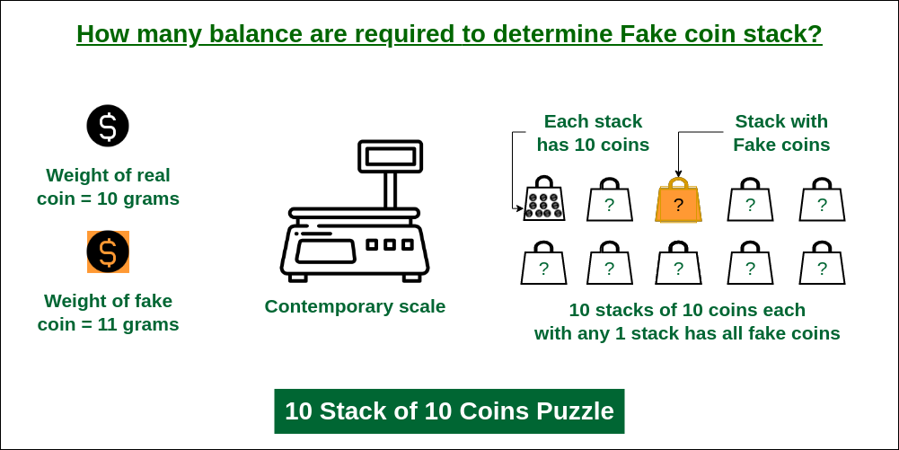
We could simply inspect every element of $\mathbf{x}$, i.e., use the canonical basis $\mathbf{A} = \mathbf{I}$ for sampling. However, this would require $n$ measurements in order to guarantee finding the non-zero entry.
You can do much better though. What if your matrix consisted of a single projection vector $\mathbf{A} = [1, 2, \ldots, n]$, which encodes each item’s position in its value? Then a single measurement would directly give you the position we are looking for!
Alright, let us make it a bit more challenging. What if you do not know the value of the non-zero entry? One measurement will not work anymore no matter how we choose $\mathbf{A}$:
- If there is a null value $A_{1j} = 0$, any signal whose non-zero element is at location $j$ will give a null measurement.
- If all values in $\mathbf{A}$ are non-zero, any vector $\mathbf{x}$ whose non-zero element at location $j$ is $x_j = \frac{1}{A_{1j}}$ will give a unitary measurement.
In other words: using a single measurement leads to an irresolvable ambiguity. What about two measurements? Our vector measurement $\mathbf{y} = [y_1, y_2]$ would correspond to a scaled version of the column $\mathbf{a}_j$, where $j$ is the position of the non-zero entry in $\mathbf{x}$. As long as no column in $\mathbf{A}$ is a multiple of another, we can uniquely identify the non-zero entry.:
- Its position $j$ would correspond to the column in $\mathbf{A}$ that is a scaled version of the measurement $\mathbf{y}$.
- Its value would be $x_j = \frac{y_1}{A_{1j}} = \frac{y_2}{A_{2j}}$.
Nonetheless, it would require $O(n)$ operations since we might have to inspect all $n$ columns in $\mathbf{A}$.
What if we know our signal has two non-zero entries? If four columns (let us use the first four to illustrate it) are linearly dependent, they would satisfy
\begin{equation} z_1 \cdot \mathbf{a}_1 + z_2 \cdot \mathbf{a}_2 + z_3 \cdot \mathbf{a}_3 + z_4 \cdot \mathbf{a}_4 = 0 \end{equation}
or equivalently
\begin{equation} z_1 \cdot \mathbf{a}_1 + z_2 \cdot \mathbf{a}_2 = - z_3 \cdot \mathbf{a}_3 - z_4 \cdot \mathbf{a}_4 = 0 \end{equation}
This means the following vectors:
\begin{equation} \mathbf{x} = [z1, z2, 0, 0, \ldots, 0] \quad \text{and} \quad \mathbf{x} = [0, 0, -z3, -z4, \ldots, 0] \end{equation}
will give us the same measurements. If we use $m=2$ or $m=3$, any four columns will necessarily be linearly dependent. Therefore, we need at least $m=4$, ensuring the sensing matrix $\mathbf{A}$ in such a way that no four columns are linearly dependent. It is unclear how to design such a matrix, but it seems drawing the columns at random would likely satisfy this condition. Furthermore, to retrieve the original signal, we might need to inspect all $\binom{n}{2}$ possible pairs of columns.
From this simple scenarios, we can observe several things:
- There is potential to recover a $k$-sparse signal from $\textbf{m} \ll \textbf{n}$ measurements.
- The number of measurements is greater than the sparsity level though, $\textbf{m} \geq \textbf{k}$
- The sensing matrix on which we project the signal cannot be the basis in which the signal is sparse. Otherwise, we would need to take $n$ samples to recover the signal. The two basis should be as decorrelated as possible.
- Design of the sensing matrix is key and randomness seems to play.
- Naive reconstruction algorithms require on the order of $\binom{\textbf{n}}{\textbf{s}}$ operations to recover the signal.
2.3. The Restricted Isometry Property (RIP)
The notion of how correlated the sensing matrix $\mathbf{C}$ is with the sparsity basis $\mathbf{\Psi}$ is captured by the coherence metric:
$$ \begin{equation} \mu(\mathbf{C}, \mathbf{\Psi}) = \sqrt{n} \max_{1\leq i,j \leq n} \lvert \mathbf{C}_i^T \cdot \mathbf{\Psi}_j \rvert \end{equation} $$
where $\mathbf{C}_i$ and $\mathbf{\Psi}_j$ are the $i$-th column of $\mathbf{C}$ and the $j$-th column of $\mathbf{\Psi}$ respectively. A small coherence means that columns in the sensing matrix spread their energy when expressed in the sparsity basis $\mathbf{\Psi}$. By taking measurements on this decorrelated matrix, we can hope to recover the signal with fewer measurements.
Example of pairs of basis that have low coherence include:
- Fourier basis and the canonical basis.
- Wavelet basis and the noiselet basis.
- Random basis and any basis.
When measurements are incoherent, we can define the isometry constant $\delta_k$ as the smallest number such that the following holds:
$$ \begin{equation} (1-\delta_k) \lVert \mathbf{s} \rVert_2^2 \leq \lVert \mathbf{C} \mathbf{\Psi} \mathbf{s} \rVert_2^2 \leq (1+\delta_k) \lVert \mathbf{s} \rVert_2^2 \end{equation} $$
which means $\mathbf{\Theta}$ almost preserves the norm of any $k$-sparse vector.
Suppose we have arbitrary $\frac{k}{2}$-sparse vectors $\mathbf{s}$. In order reconstruct such vectors from measurements $\mathbf{y} = \mathbf{\Theta} \mathbf{s}$, we must be able to distinguish between measurements $\mathbf{y}_1 = \mathbf{\Theta} \mathbf{s}_1$ and $\mathbf{y}_2 = \mathbf{\Theta} \mathbf{s}_2$ of any two such vectors. If $\mathbf{y}_1 = \mathbf{y}_2$ for two different $\mathbf{s}_1 \neq \mathbf{s}_2$, then retrieval becomes unfeasible.
The difference vector $\mathbf{s} = \mathbf{s}_1 - \mathbf{s}_2$ between $\frac{k}{2}$-sparse vectors is at most a $k$-sparse vector. The RIP property ensures that the measurements will be distinct enough to allow for the reconstruction of the original signals.
Importantly, if the RIP holds, it can be proven that:
- If $\delta_{2k} (\mathbf{\Theta}) < 1$, then we can find $\mathbf{s}$ as the unique solution to the $l_0$-norm minimization problem.
- If $\delta_{2k} (\mathbf{\Theta}) < \sqrt{2} - 1$, then we can find $\mathbf{s}$ as the unique solution to the $l_1$-norm minimization problem.
3. Why does the L1- norm work?
As we have already mentioned, the $l_0$-norm minimization problem is non-convex and NP-hard. However, under certain conditions, it is possible to relax it to a convex $l_1$-norm minimization problem. This is a remarkable result, and it is not immediately clear why the $l_1$-norm, and not any other norm, like the $l_2$-norm, is a good proxy for sparsity. All the code used to generate the animations in this section is available at the following public repository:
To try to understand this, let us start by stating the optimization problem we are trying to solve in the noisy scenario:
$$ \begin{equation} \min_{\mathbf{s}} \lVert \mathbf{s} \rVert_1 \quad \text{subject to} \quad \lVert \mathbf{y} - \mathbf{\Theta} \mathbf{s} \rVert_2 \leq \epsilon \end{equation} $$
By introducing a Lagrange multiplier $\beta$, we can rewrite the problem in its LASSO form:
$$ \begin{equation} \min_{\mathbf{s}} \lVert \mathbf{y} - \mathbf{\Theta} \mathbf{s} \rVert_2^2 \quad \text{subject to} \quad \lVert \mathbf{s} \rVert_1 \leq \beta \end{equation} $$
Lagrange Multiplier
Let us say we are tasked with finding the solution for constrained optimization problem given by $$ \begin{equation} \min_{\mathbf{x}} \mathbf{g} (\mathbf{x}) \quad \text{subject to} \quad \mathbf{f} (\mathbf{x}) \leq \beta \end{equation} $$ We can visualize the problem for the 2D case. To do so, we will draw the region $\mathbf{f} (\mathbf{x}) \leq \beta$ shaded in blue. Then we can draw the isocontours of the function $\mathbf{g} (\mathbf{x})$ in red. For the sake of the argument, we will draw three different contours: one that intersects with the blue region, one that is tangent to it and one that lies outside of it.
- The solution cannot lie along $\mathbf{f} (\mathbf{x}) = \alpha_1$. That would imply it is outside the blue region and therefore it would not satisfy the constraint.
- The solution cannot lie $\mathbf{f} (\mathbf{x}) = \alpha_3$. It would satisfy the constraint, but the isocontour intersects with the blue region. That means it is possible to move to an adjacent contour that lies inside the blue region and has a lower value of $\mathbf{g} (\mathbf{x})$.
- The solution lies at the point of tangency between the isocontour and the blue region. This is the point that minimizes $\mathbf{g} (\mathbf{x})$ while satisfying the constraint.
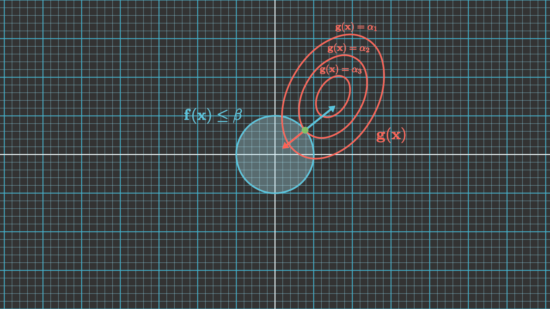
At the point of tangency, the gradient both functions must be parallel but pointing in opposite directions. That means $$ \begin{equation} \nabla \mathbf{g} (\mathbf{x}) = - \lambda \nabla \mathbf{f} (\mathbf{x}) \end{equation} $$ for some positive scalar $\lambda$. This is the Lagrange multiplier.
We can therefore rewrite the optimization problem as $$ \begin{equation} \min_{\mathbf{x}} \mathbf{h} (\mathbf{x}) = \min_{\mathbf{x}} \mathbf{g} (\mathbf{x}) + \lambda \mathbf{f} (\mathbf{x}) \end{equation} $$ Why is that? Well, to find the solution to an optimization problem, we need to find the point at which the gradient of the cost function $\mathbf{h} (\mathbf{x})$ is zero: $$ \begin{equation} \nabla \mathbf{h} (\mathbf{x}) = \nabla \mathbf{g} (\mathbf{x}) + \lambda \nabla \mathbf{f} (\mathbf{x}) = 0 \end{equation} $$ which is equivalent to the previous equation.
Last, this reasoning will allow us to revert the two terms in the original optimization problem. We can rewrite it as $$ \begin{equation} \min_{\mathbf{x}} \mathbf{f} (\mathbf{x}) \quad \text{subject to} \quad \mathbf{g} (\mathbf{x}) \leq \epsilon \end{equation} $$ So to sum up, there exist some scalars $\lambda$, $\beta$ and $\epsilon$ such that the solution to the three problems is the same.
The isocontours for the $l_2$-norm term we are trying to minimize are concentric $N$-dimensional ellipsoids centered at $\mathbf{y}$. On the other hand, the $l_1$-norm constraint is an $N$-dimensional diamond centered at the origin. The solution to the optimization problem is therefore the point for which one of the ellipsoids is tangent to the diamond, as depicted in the figure below for the 2D case.

Let us focus for simplicity in the illustrated 2D scenario. Notice that, for a given slope $m$, the line that passes through the points of tangency for a set of concentric ellipses is a straight line that goes through the center of those ellipses. We will refer to this line as the secant line of tangency.
Tangent to an ellipse
We will make the following derivation for an ellipse centered at the origin and aligned with the canonical basis. That is general enough though, since any other ellipse can be transformed into such one. It would then suffice to revert the shift and rotation on the outcomes. The equation for an ellipse is given by: $$ \begin{equation} \frac{x^2}{a^2} + \frac{y^2}{b^2} = 1 \end{equation} $$ where $a$ and $b$ are the semi-major and semi-minor axes of the ellipse.We can compute the derivative of the ellipse with respect to $x$: $$ \begin{equation} \frac{dy}{dx} = \pm \frac{b}{a} \frac{x}{\sqrt{a^2-x^2}} \end{equation} $$ We are interested in the point of tangency for a given slope $m$. That means the derivative of the ellipse at that point should be equal to the slope of the line: $$ \begin{equation} m = \pm \frac{b}{a} \frac{x_0}{\sqrt{a^2-x_0^2}} \rightarrow m^2 = \frac{b^2}{a^2} \frac{x_0^2}{a^2-x_0^2} \end{equation} $$ We can solve this equation to find the $x_0$ coordinate of the point of tangency: $$ \begin{equation} x_0 = \pm \frac{a^2 m^2}{\sqrt{a^2 m^2 + b^2}} \end{equation} $$ We can then find the $y_0$ coordinate by substituting this value into the equation of the ellipse: $$ \begin{equation} y_0 = \pm \frac{b^2}{\sqrt{a^2 m^2 + b^2}} \end{equation} $$ This allows to express the tangent line as $$ \begin{equation} y = mx \pm \sqrt{a^2 m^2 + b^2} \end{equation} $$
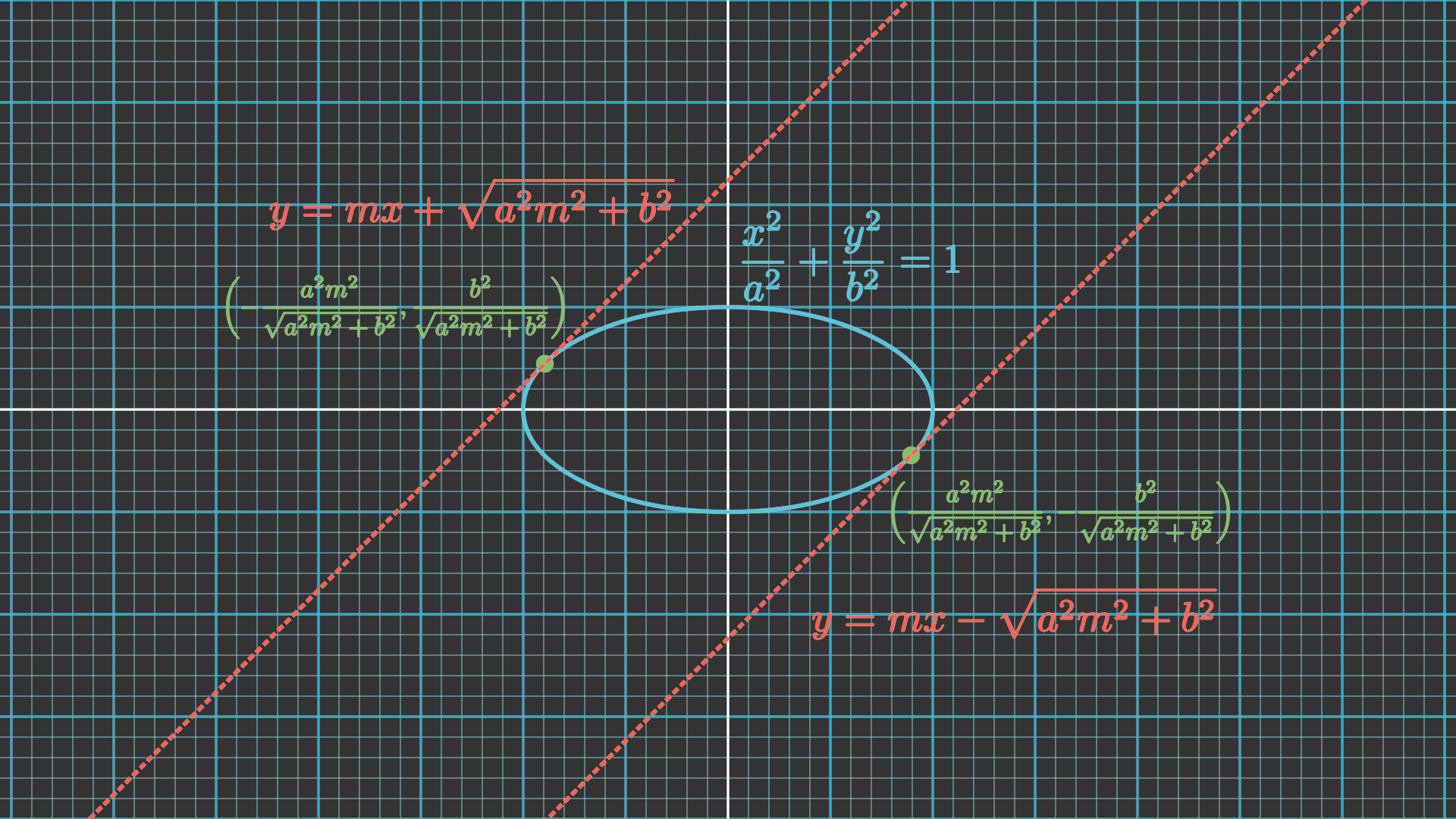
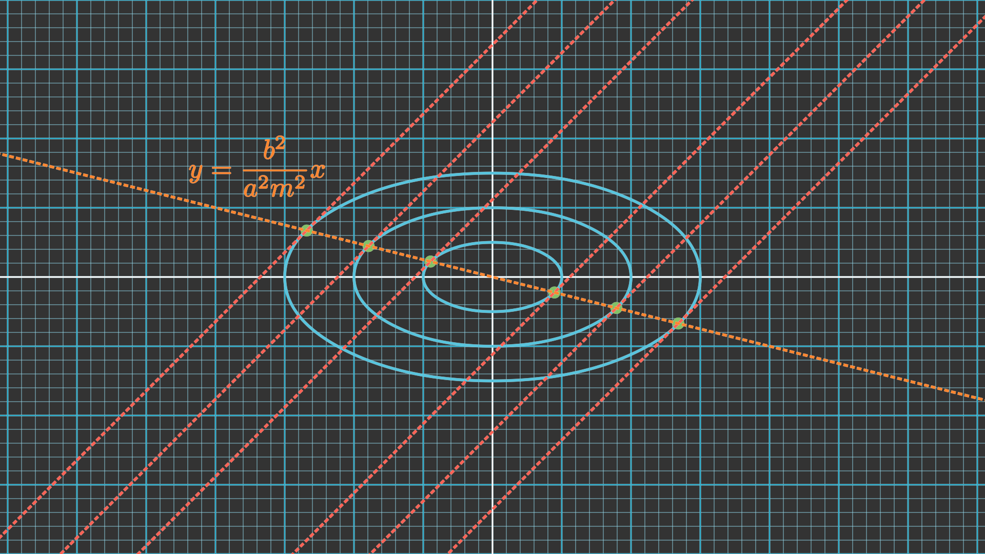
The orientation and aspect ratio of this set of concentric ellipses is given by matrix $\mathbf{\Theta}$, whereas its center is given by the vector $\mathbf{y}$. That means the solution to the optimisation problem will lie along:
- The edges of the $l_1$-ball: only if the secant line of tangency for the concentric ellipses intersects with it. In that case, it will have two non-zero elements.
- The edges of the $l_1$-ball: otherwise. In that case, it will have only one non-zero element.
Consequently, the solution will be sparse whenever it lies on the vertices of the diamond. How likely is this to happen? Well, let us see how different transforms to the set of ellipses impact the solution (we skip scaling since it results in the same set):
- Shift
- Rotation
- Aspect ratio variation
We can observe how the solution to the optimization problem is highly dependent on the orientation and aspect ratio of the set of concentric ellipses. Most often, the secant line of tangency will not intersect with the diamond, leading the solution to lie in one of its vertices and therefore be sparse.
The reason the $l_1$-norm works as a proxy for sparsity is because of its discontinuities at the vertices. They create a skewed landscape that makes the solution gravitate towards those vertices more often than not. This is not the case for the $l_2$-norm, which does not have any preferential point along its smooth surface, as the following videos summarizes.
How about the 3D case? The reasoning is analogous:
- If the secant line of tangency intersects with one of the faces of the diamond, the solution will have three non-zero elements.
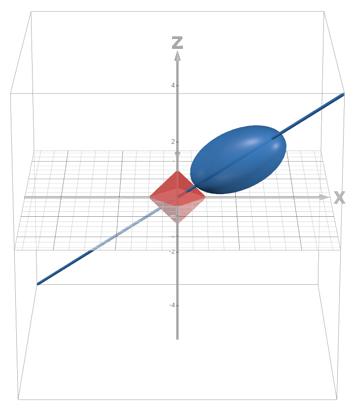
Example of a scenario where the solution lies in the face of the diamond. - If the secant line of tangency intersects does not intersect with the faces, then it boils down to the 2D plane in which the closest edge lives, which we have already explained earlier. In particular, we care about the ellipse resulting from the intersection between the ellipsoid and that plane:
- If the secant line of tangency for the ellipse intersects with one of the edges of the diamond, the solution will have two non-zero elements.
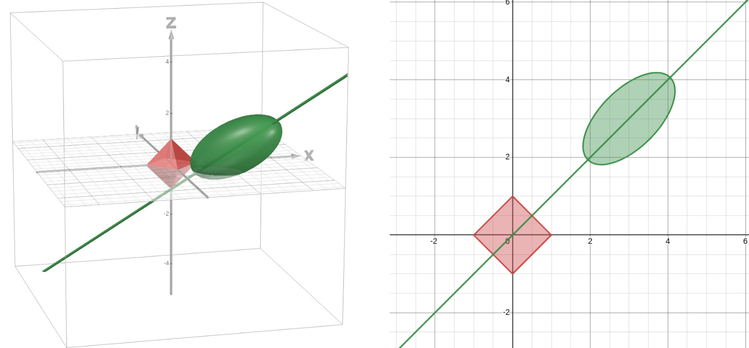
Example of a scenario where the solution lies in the edge of the diamond. - If the secant line of tangency does not intersect with any edgee, then the solution goes to the vertex of the diamond and will have only one non-zero element.
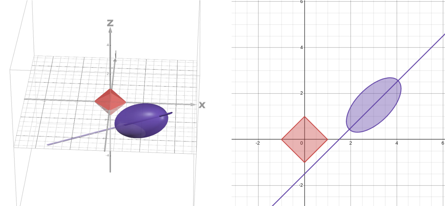
Example of a scenario where the solution lies in the vertex of the diamond.
- If the secant line of tangency for the ellipse intersects with one of the edges of the diamond, the solution will have two non-zero elements.
It is not possible to visually illustrate this process beyond the 3D case. However, the reasoning is the same and it gives us a good intuition of why the $l_1$-norm is a good proxy for sparsity.
4. Conclusion
In this post:
- We have introduced the concept of compressed sensing and discussed the conditions under which it is possible to recover a sparse signal from a set of linear measurements.
- We have seen that the key to successful recovery is the incoherence between the sensing matrix and the sparsity basis.
- We have discussed the Restricted Isometry Property and the role of the $l_1$-norm in the recovery process.
- We have shown that the $l_1$-norm is a good proxy for sparsity because of the discontinuities of the $l_1$-ball. This makes the solution gravitate towards a sparse solution.
5. References
- E. Candes, M.B. Walkin (2008), Signal Processing Magazine, IEEE 25 (2), 21-30. An Introduction To Compressive Sampling
- D. Donoho (2006), IEEE Transactions on Information Theory, 52(4), 1289-1306. Compressed Sensing
- S.L. Brunton, J.L. Proctor, J.N. Kutz (219), Cambridge. Data-driven science and engineering: machine learning, dynamical systems, and control
- S. Wright (2009), SIAM Gator Student Conference, Gainesville, March 2009. Optimization Algorithms for Compressed Sensing
- K. Scheinberg (2017), University of Lehigh. Lecture on Sparse Convex Optimization
- Tangents of an ellipse